Using garch to learn a little about the distribution of returns.
Previously
There are posts on garch — in particular:
- A practical introduction to garch modeling
- The components garch model in the rugarch package
- garch and long tails
There has also been discussion of the distribution of returns, including a satire called “The distribution of financial returns made simple”.
Question
Volatility clustering affects the distribution of returns — the high volatility periods make the returns look longer tailed than if we take the volatility clustering into account.
The question we try to sneak up on is: What is the distribution of returns when volatility clustering is accounted for? More specifically, what is the distribution using a reasonable garch model?
Data
Daily log returns of 443 large cap US stocks with histories from the start of 2004 into the first few days of 2013 were used. There were 2267 days of returns for each stock.
The components garch model assuming a t distribution was fit to each stock.
Results
Actual results
The estimated degrees of freedom for the stocks is shown in Figure 1. Estimation failed for one stock.
Figure 1: Estimated degrees of freedom for the t in the components garch model for the US large cap stocks. 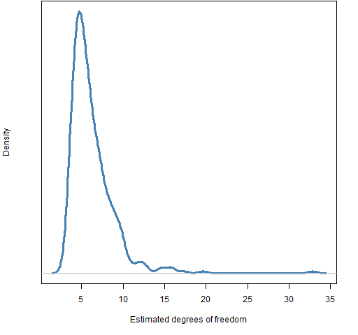 A lot of the estimates are close to 6 and hardly any (about 5%) are greater than 10.
Normal distribution
Next was to see what degrees of freedom are estimated if the residuals are normally distributed. The fits from the first three stocks were used — separately — to simulate series (200 each) and then fit the model to those simulated series.
Figure 2 shows the distributions of the estimated degrees of freedom from the three fits.
Figure 2: Distributions of estimated degrees of freedom using the initial simulated series from three fits. 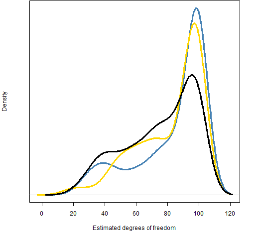 I’m hoping that we can all agree that the normal distribution can be ruled out as the actual distribution. There is virtually no overlap between the distribution in Figure 1 and those in Figure 2.
It appears that the black distribution in Figure 2 is different from the other two — that it has a much higher probability of being less than 80. But the distributions are based on only 200 series each; there will be noise. A further 1000 series were generated for each fit to see if the pattern persists with new, more extensive data. Figure 3 shows the results.
Figure 3: Distributions of estimated degrees of freedom using the confirmatory simulated series from three fits. 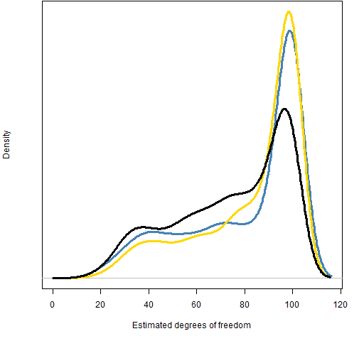 The distributions do indeed appear to be different — the black one has just over 50% probability of being less than 80 while the other two have less than 40%.
This means that we can’t assume that the estimate of the degrees of freedom is independent of the other parameters.
t distribution
The next test was — for each stock — simulate a series using the coefficients estimated for the stock but with residuals following a t distribution with 6 degrees of freedom. The distribution of estimated degrees of freedom from fitting the simulated series is shown in Figure 4.
Figure 4: Distribution of estimated degrees of freedom for series created with a t with 6 degrees of freedom and coefficients specific to each stock. 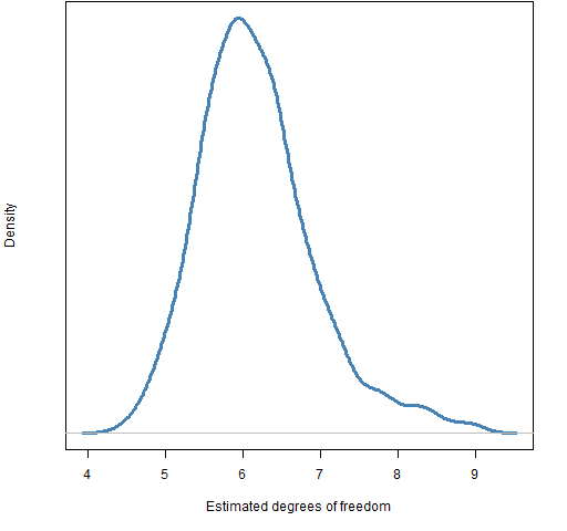 This is much too centered near 6 compared to Figure 1. About 20% of the real estimated degrees of freedom are smaller than the smallest degree of freedom estimated from the t6 simulations. Likewise, about 10% of the real degrees of freedom are bigger than the biggest from the t6 simulations.
I propose two (not necessarily mutually exclusive) possibilities:
- Different stocks have different distributions
- The real distribution is not t and the degrees of freedom are not a good approximation
Summary
We’ve shown — once again — that the normal distribution is not believable.
We’ve also highlighted our ignorance about the true situation.
Appendix R
The R language was used to do the computing.
collect coefficients from the model on stocks
We start by making sure the rugarch package is loaded in the session, create the specification object that we want, and fit garch models to the first three stocks:
require(rugarch)

comtspec <- ugarchspec(mean.model=list(
  armaOrder=c(0,0)), distribution="std",
  variance.model=list(model="csGARCH"))
fit1 <- ugarchfit(spec=comtspec, initret[,1])
fit2 <- ugarchfit(spec=comtspec, initret[,2])
fit3 <- ugarchfit(spec=comtspec, initret[,3])
The initret object is the matrix of returns. Next we create a matrix to hold the coefficients for all of the stocks:
gcoefmat <- array(NA, c(443, length(coef(fit1))),
   list(colnames(initret),names(coef(fit1))))
That the matrix is initialized with missing values is not accidental. We’re not guaranteed that the default estimation will work. Now we’re ready to collect the coefficients:
for(i in 1:443) {
  thiscoef <- try(coef(ugarchfit(spec=comtspec, initret[,i])))
  if(!inherits(thiscoef, "try-error") && length(thiscoef) == 7) {
    gcoefmat[i,] <- thiscoef
  }
  cat("."); if(i %% 50 == 0) cat("\n")
}
cat("\n")
This takes evasive action in case we don’t get a vector of coefficients like we expect — it uses the try function to continue going even if there is an error. It also gives an indication of how far along the loop is (since fitting over 400 garch models is not especially instantaneous).
simulate garch from a specific distribution
Here is a function that will take a garch fit object and simulate a number of series using residuals from a particular distribution:
pp.garchDistSim <- function(gfit, FUN, trials=200,
   burnIn=100, ...)
{
  # simulate a garch model given a fit

  # placed in the public domain 2013 by Burns Statistics

  # testing status: untested

  ntimes <- gfit@model$modeldata$T
  FUN <- match.fun(FUN)
  inresid <- scale(matrix(FUN((ntimes+burnIn) * trials,
       ...), ntimes+burnIn, trials))
  simseries <- ugarchsim(gfit, n.sim=ntimes,
       n.start=burnIn, m.sim=trials,
       startMethod="sample", custom.dist=list(name="sample",
       distfit = inresid))@simulation$seriesSim
  simseries
}
The residuals that are given to the simulation function are scaled (with the scale function) to have zero mean and variance 1 because the routine expects the residuals to be distributed like that. It can get grumpy if that is obviously not the case.
simulate with normals
The function above is used like:
gsnorm1 <- pp.garchDistSim(fit1, rnorm, trials=200)
gsnorm2 <- pp.garchDistSim(fit2, rnorm, trials=200)
gsnorm3 <- pp.garchDistSim(fit3, rnorm, trials=200)
Once we have these series, we can fit the garch model to them and save the coefficients:
gsnorm1.coefmat <- array(NA, c(200, 7),
   list(NULL, names(coef(fit1))))
gsnorm2.coefmat <- gsnorm3.coefmat <- gsnorm1.coefmat

for(i in 1:200) {
  thiscoef <- try(coef(ugarchfit(spec=comtspec, gsnorm1[,i])))
  if(!inherits(thiscoef, "try-error") && length(thiscoef) == 7) {
    gsnorm1.coefmat[i,] <- thiscoef
  }
  cat("."); if(i %% 50 == 0) cat("\n")
}
cat("\n")
difference of distributions from normal
We can get the confidence interval for the proportion of the black distribution from the confirmatory normal estimates being less than 80 by using the binom.test function:
> binom.test(sum(gsnorm2M.coefmat[,7] < 80, na.rm=TRUE),
+            sum(!is.na(gsnorm2M.coefmat[,7])))

	Exact binomial test

data:  sum(gsnorm2M.coefmat[, 7] < 80, na.rm = TRUE)
  and sum(!is.na(gsnorm2M.coefmat[, 7]))
number of successes = 489, number of trials = 963,
  p-value = 0.6519
alternative hypothesis: true probability of success is
  not equal to 0.5
95 percent confidence interval:
 0.4757106 0.5398179
sample estimates:
probability of success
             0.5077882
That the binomial test sees 963 observations means that 37 of the 1000 series didn’t produce an appropriate vector of coefficients using the default fitting settings.
The stock that is the odd one out (the black one) is ABT. The other two are MMM and ANF. The fit for ABT is significantly more persistent than for the other two (but experimentation is needed to understand what is happening).
simulate given a garch specification
Here is a function that simulates series given a garch specification:
pp.gspecDistSim <- function(spec, FUN, ntimes, trials=1,
 burnIn=100, ...)
{
  # simulate a garch model given a specification

  # placed in the public domain 2013 by Burns Statistics

  # testing status: untested

  FUN <- match.fun(FUN)
  inresid <- scale(matrix(FUN((ntimes+burnIn) * trials, ...),
     ntimes+burnIn, trials))
  simseries <- ugarchpath(spec, n.sim=ntimes,
     n.start=burnIn, m.sim=trials, startMethod="sample",
 custom.dist=list(name="sample",
     distfit = inresid))@path$seriesSim
  simseries
}
paired simulation with a t
The function immediately above was used like:
gst6specific.coefmat <- array(NA, c(443, 7),
   dimnames(gcoefmat))
for(i in 1:443) {
  thisspec <- comtspec
  stockcoef <- gcoefmat[i,]
  if(any(is.na(stockcoef))) next
  setfixed(thisspec) <- as.list(stockcoef)
  simser <- pp.gspecDistSim(thisspec, rt, ntimes=2267,
     trials=1, df=6)
  thiscoef <- try(coef(ugarchfit(spec=comtspec, simser)))
  if(!inherits(thiscoef, "try-error") && length(thiscoef) == 7) {
    gst6specific.coefmat[i,] <- thiscoef
  }
  cat("."); if(i %% 50 == 0) cat("\n")
}
cat("\n")
Note that the call to pp.gspecDistSim in this loop is using R’s dot-dot-dot mechanism.

David Ardia points out that he has a paper doing something similar: http://papers.ssrn.com/sol3/papers.cfm?abstract_id=2226406
Pingback: Blog year 2013 in review | Portfolio Probe | Generate random portfolios. Fund management software by Burns Statistics