Task
Optimize an asset allocation where we want weights rather than units (like shares or contracts).
Preparation
- vector of expected returns
- variance matrix for the assets
- Portfolio Probe
You need a variance matrix of the asset returns, and an expected return for each asset.
We assume that transaction costs are not an issue, in which case optimizing the trade is the same as optimizing the entire portfolio. (If this assumption is not right, then the existing portfolio and trading costs can be added.)
You also need to have the Portfolio Probe package loaded into your R session:
require(PortfolioProbe)
If you don’t have Portfolio Probe, see “Demo or Buy”.
Doing the example
xaLWvar06variance matrix from “Returns to variance matrix” examplexaMACDmatrix from “Compute a technical indicator” example to use for expected returns
Doing it
We’ll do three optimizations:
- maximize the information ratio given weight constraints
- maximize a mean-variance utility given weight constraints
- maximize the information ratio given risk fraction constraints
We need to do a few things before we get to the optimization.
Asset allocation problems are generally done with a few to a few dozen assets. In that light we will use only the first 10 assets in the example data.
Preliminaries
The inputs we need in order to get our optimal portfolio are:
- variance matrix of the asset returns
- vector of expected returns
- vector to use as “prices”
- amount of “money” in the portfolio
- appropriate constraints
variance and expected returns
We can extract the part of the variance matrix that we want to use and scale it with:
aaVar <- xaLWvar06[1:10,1:10] * 10000 * 252
Likewise, we can get a portion of the MACD signal object to use as our vector of expected returns:
aaExpRet <- xaMACD[251,1:10] + 2
We can look at the expected returns and their volatilities with:
> aaExpRet
    XA101     XA103     XA105     XA107     XA108
2.9178291 2.9114743 3.1844481 2.8825741 3.4268342
    XA111     XA113     XA115     XA120     XA126
1.6649796 0.4527979 2.8888312 3.1706957 0.7013360
> sqrt(diag(aaVar))
   XA101    XA103    XA105    XA107    XA108
15.09122 29.12268 16.67386 13.56991 22.95124
   XA111    XA113    XA115    XA120    XA126
22.35138 24.27847 36.34904 18.60758 33.68222
prices and value
The optimizer presumes that we have assets at a certain price per unit and that we have some given amount of money to put into the portfolio. With asset allocation we are ignoring (or ignorant of) the available amount of money. Plus the assets are often abstractions and don’t have a specific price.
Hence we need to trick the optimizer. The first part of the trick is to give each asset a price of 1:
aaPrice <- rep(1, 10)
names(aaPrice) <- names(aaExpRet)
This price vector looks like:
> aaPrice
XA101 XA103 XA105 XA107 XA108 XA111 XA113 XA115
    1     1     1     1     1     1     1     1
XA120 XA126
    1     1
Part two of the trick is to say how much “money” to put as the gross value of the portfolio. This could be anything, but a convenient quantity is 10,000. This will give us weights to the nearest basis point.
> aaGross <- 10000 + c(-.5, .5)
> aaGross
[1]  9999.5 10000.5
We’ve created a length two vector that describes a range with exactly one integer in it. We’ll use this as the allowable range for the gross value of the portfolio. Since the optimizer trades integer amounts, the sum of the units in the portfolio will sum to that integer.
Optimization: information ratio with weight constraints
We’re now ready to do an optimization. The only constraint that we impose besides the gross value and being long-only is that no asset has a weight bigger than 20%.
aaMaxInfoWt <- trade.optimizer(aaPrice, variance=aaVar,
   expected.return=aaExpRet, gross=aaGross,
   long.only=TRUE, max.weight=.2)
We are not specifying what utility to use, so it will use the default which is to maximize the information ratio.
Optimization: mean-variance utility with weight constraints
If we are using a mean-variance utility, we need to decide what risk aversion to use.
aaMeanVarWt <- trade.optimizer(aaPrice, variance=aaVar,
   expected.return=aaExpRet, gross=aaGross,
   long.only=TRUE, max.weight=.2,
   utility="mean-variance", risk.aversion=4)
We’ve added two arguments to the previous optimization. We use the utility argument to state the form of utility to use, and we use the risk.aversion argument to state the risk aversion that we want to use.
Note that the form of the utility is: expected return minus risk aversion times variance. Some have a one-half in the last term.
Optimization: information ratio with risk fraction constraints
In this case we switch to a constraint that is probably better.
aaMaxInfoRf <- trade.optimizer(aaPrice, variance=aaVar,
   expected.return=aaExpRet, gross=aaGross,
   long.only=TRUE, risk.fraction=.2)
This is just like the first optimization except that we say “risk.fraction” instead of “max.weight”.
Print results
The resulting (first) object is printed like:
> aaMaxInfoWt
$new.portfolio
XA101 XA103 XA105 XA107 XA108 XA120
 2000    56  2000  2000  1944  2000

$trade
XA101 XA103 XA105 XA107 XA108 XA120
 2000    56  2000  2000  1944  2000

$results
 objective    negutil       cost    penalty
-0.3150499 -0.3150499  0.0000000  0.0000000

$converged
[1] TRUE

$objective.utility
[1] "information ratio"

$alpha.values
     A0
3.11359

$var.values
      V0
97.67069

$utility.values
[1] -0.3150499

$existing
NULL

$violated
NULL

$timestamp
[1] "Wed Sep 26 18:47:11 2012"
[2] "Wed Sep 26 18:47:13 2012"

$call
trade.optimizer(prices = aaPrice, variance = aaVar, expected.return = aaExpRet,
    gross = aaGross, long.only = TRUE, max.weight = 0.2)
(There are some additional components to the object that are not shown.)
From the first component we see that 4 assets are at the maximum weight.
Explanation
Weights
Let’s play with the optimal portfolio from the first optimization:
> aaNewPort1 <- aaMaxInfoWt$new.portfolio
> aaNewPort1
XA101 XA103 XA105 XA107 XA108 XA120
 2000    56  2000  2000  1944  2000
> sum(aaNewPort1)
[1] 10000
> aaNewPort1 / sum(aaNewPort1)
 XA101  XA103  XA105  XA107  XA108  XA120
0.2000 0.0056 0.2000 0.2000 0.1944 0.2000
We see that the sum of the quantities for all the assets in the portfolio is 10,000 (as we should expect). We can get the weights by dividing by 10,000. A confirmation of this is to get the weights by another means:
> valuation(aaMaxInfoWt)$weight
 XA101  XA103  XA105  XA107  XA108  XA120
0.2000 0.0056 0.2000 0.2000 0.1944 0.2000
Constraints
The first two optimizations constrain the maximum weight of the assets to 20%. The last optimization constrains the maximum fraction of portfolio variance attributed to an asset to 20%.
The latter constraint is much more likely to be what you really want. However, the technology to do that didn’t used to be available so weight constraints were used as a cheap substitute.
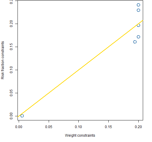
Figure 1 compares the optimal weights from the two information ratio optimizations. They both give a lot of weight to the same five assets, and they both have trivial weights in the same sixth asset. The key difference is that the risk fraction optimization varies the weights of the big-five assets so they all contribute roughly equal amounts of risk.
Figure 1: The weights of the six assets that are in aaMaxInfoWt and aaMaxInfoRf. 
Further details
We gave the max.weight and risk.fraction arguments a single number. This means that all of the assets have that same number as their constraint. It is also possible to give those arguments a vector with separate constraints for each asset.
For example we could give either (or both) of those arguments the vector:
> aaConstr <- .2 * aaPrice
> aaConstr[c(1,9)] <- .1
> aaConstr
XA101 XA103 XA105 XA107 XA108 XA111 XA113 XA115
  0.1   0.2   0.2   0.2   0.2   0.2   0.2   0.2
XA120 XA126
  0.1   0.2
This would constrain two of the assets more than the others.
See also
Navigate
- Back to “Optimize Trades”
- Back to the top level of “Portfolio Probe Cookbook”
