Task
Include trading costs in an optimization.
Preparation
This presumes that you can do a basic portfolio optimization. For example, that you have mastered “Passive, no benchmark (minimum variance)”.
- Portfolio Probe
You need to have the Portfolio Probe package loaded into your R session:
require(PortfolioProbe)
If you don’t have Portfolio Probe, see “Demo or Buy”.
Doing the example
- The objects:
priceVector,grossVal,curPortfolthat are defined in several examples, such as in “Passive, no benchmark (minimum variance)” xaLWvar06variance matrix from “Returns to variance matrix” example
Doing it
We will do optimizations that:
- impose simplistic linear costs
- impose simplistic linear costs that differ for buying and selling
- impose non-linear costs
None of the examples are complete — see the “Further details” section for the missing ingredient.
Simplistic linear costs
We perform an optimization that assumes that trading costs are 10 basis points:
opTC10bps <- trade.optimizer(priceVector,
   variance=xaLWvar06, existing=curPortfol,
   gross=grossVal, long.only=TRUE,
   utility="minimum variance",
   long.buy.cost=0.001 * priceVector)
This optimization is correct in the sense that it tells the optimizer that trading costs are 10 basis points. But the optimization is (almost surely) wrong in the sense of doing the right thing even if trading costs really are 10 basis points — see the “Further details” section below.
Costs that differ for buying and selling
Real costs are different depending on whether you are buying or selling. In a long-only portfolio you merely do a sell. But when you buy, you are also committing yourself to a subsequent sell.
Here we impose 20 basis point costs for buying and 10 basis points for selling:
opTC2010bps <- trade.optimizer(priceVector,
   variance=xaLWvar06, existing=curPortfol,
   gross=grossVal, long.only=TRUE,
   utility="minimum variance",
   long.buy.cost=0.002 * priceVector,
   long.sell.cost=0.001 * priceVector)
Non-linear costs
The cost of small trades is linear, but bigger trades have market impact and grow faster than linear. Suppose that we believe that market impact grows with an exponent of 0.6 — so slightly faster than the square root of the inventory model.
First we want to create a two-column matrix that holds the trading cost coefficients per asset. A quick stand-in is:
tcNonlin <- cbind(priceVector * .001,
   rep(1:5, length=350) * .005)
This looks like:
> head(tcNonlin)
         [,1]  [,2]
XA101 0.03356 0.005
XA103 0.07225 0.010
XA105 0.07439 0.015
XA107 0.19206 0.020
XA108 0.00591 0.025
XA111 0.01598 0.005
Now we are ready to do the optimization:
opTCnonlin <- trade.optimizer(priceVector,
   variance=xaLWvar06, existing=curPortfol,
   gross=grossVal, long.only=TRUE,
   utility="minimum variance",
   long.buy.cost=tcNonlin, cost.par=c(1, 1.6))
Explanation
Linear costs
The value given as long.buy.cost (and mates) should be a vector with names that are the asset identifiers. All of the tradable assets must be included. A one-column matrix also works.
There is, of course, no reason that the costs need to be proportional to prices.
Non-linear costs
The cost.par argument is a vector of the exponents that go with each column of the cost arguments (long.buy.cost and its mates). (But see the “Further details” section below.)
In the example we had:
long.buy.cost=tcNonlin, cost.par=c(1, 1.6)
with
> head(tcNonlin, 3)
         [,1]  [,2]
XA101 0.03356 0.005
XA103 0.07225 0.010
XA105 0.07439 0.015
If asset XA101 trades 99 shares (buy or sell), then the cost for it will be:
> 0.03356 * 99 + 0.005 * 99 ^ 1.6
[1] 11.1205
The numbers in the first column of long.buy.cost go with the first element of cost.par. The second column goes with the second element of cost.par, and so on. You can have as many columns as you like. In particular, there can be an element of cost.par that is zero, which means there is a fixed cost for trading the asset at all.
Buys versus sells
The full set of cost coefficient arguments is:
long.buy.costlong.sell.costshort.buy.costshort.sell.cost
Ones that are not given will default to the value of long.buy.cost (hence if you are giving costs, you always want to give this argument).
If cost.par is given, then all four of these arguments need to have the same number of columns. The number of columns, of course, has to be the length of cost.par.
Further details
Costs relative to utility
In the examples we are minimizing variance. In this case it is easy to see that we must be missing something even if we exactly reproduce our trading costs.
The cost (divided — by default — by the gross value of the portfolio) is added to the utility. So we are adding dollars to something to do with squared returns. Without costs we get the same thing whether the variance is for daily returns or for returns in percent and annualized. But we get an entirely different effect if we add the same costs in these two cases.
Portfolio Probe has the ucost argument (that defaults to 1) which scales the cost before it is put into the utility. So you might include something like:
ucost = 0.002
as an argument in an optimization.
We can do some exploration using the first optimization. The default value of ucost is 1 so that is its value with that first optimization. We can redo the optimization setting ucost to zero (that is, no trading costs):
opTC0 <- update(opTC10bps, ucost=0)
Now we can get the turnover for optimizations that have intermediate values of ucost:
turnTC <- numeric(5)
for(i in 1:5) {
   turnTC[i] <- valuation(update(opTC10bps, ucost=2^-i),
      trade=TRUE, collapse=TRUE)
}
names(turnTC) <- 2^-(1:5)
Now we can add the turnover for the two portfolios that we already have:
turnTCall <- c("1"=unname(valuation(opTC10bps,
   trade=TRUE, collapse=TRUE)), turnTC,
   "0"=unname(valuation(opTC0, trade=TRUE,
   collapse=TRUE)))
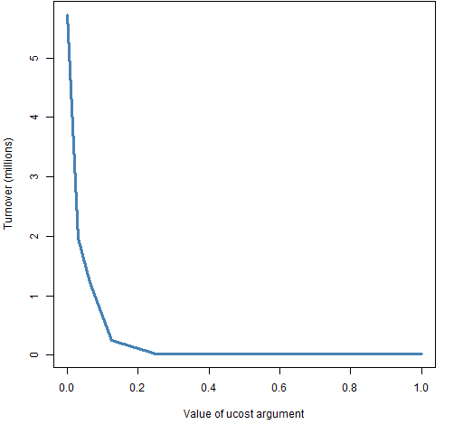
Figure 1 is a cleaned up version of:
plot(as.numeric(names(turnTCall)), turnTCall, type="l")
Figure 1: Turnover versus ucost value for the simplistic linear costs. 
The drop in the amount of trading stops at ucost=.25. So it appears in this example that ucost should be less than .25 (and larger than zero). Remember that if we change the scaling of the variance, then ucost needs to change as well.
An element of melding costs into the utility is that the costs need to be amortized. That is, the expected holding period makes a difference. You need to get a higher rate of value out of an asset that you expect to hold for a day as opposed to an asset you expect to hold for a decade.
Non-linear costs
asset-specific exponents
Above it was stated that cost.par was to be a vector. Actually it can be a matrix with rows that correspond to assets and as many columns as long.buy.cost. For example, we might give a matrix like the following to the cost.par argument:
> head(tcCostpar)
      [,1] [,2]
XA101    1 1.57
XA103    1 1.75
XA105    1 1.47
XA107    1 1.59
XA108    1 1.75
XA111    1 1.72
If all of the rows were equal, then it would be just the same as giving cost.par a vector equal to one of the rows.
per trade versus per share
The exponent that you want to use depends on what coefficients you have. The calculation done in the optimizer is on the trade as a whole — it sees the number of shares traded.
If your coefficients are from a model of trade size with an exponent of 0.6, then put 0.6 into cost.par. (Hint: I don’t think so, the exponent should be greater than 1.)
However, if the coefficients you have is for the cost per share, then you need to do a little elementary calculus to get the cost per trade size and the exponent is going to be 1.6 (the original exponent plus one).
Troubleshooting
- Is a reasonable value of
ucostgiven to match the trading costs to the utility?
- If you have non-linear costs, are the coefficients and exponents correctly matched in regards to per share versus total shares?
See also
- Control turnover for an easier way to control the amount of trading
- Example data
- Some hints for the R beginner
- the Portfolio Probe User’s Manual
Navigate
- Back to “Optimize Trades”
- Back to the top level of “Portfolio Probe Cookbook”
