A herd of heuristic algorithms is compared using a portfolio optimization.
Previously
“A comparison of some heuristic optimization methods” used two simple and tiny portfolio optimization problems to compare a number of optimization functions in the R language.
This post expands upon that by using a portfolio optimization problem that is of a realistic size (but still with an unrealistic lack of constraints).
Test case
The optimization problem is to select 30 assets out of a universe of 474 and find their best weights. The weights must be non-negative and sum to 1. The integer constraint is binding — more than 30 assets in the portfolio can give a better utility. The utility is mean-variance.
Each optimizer was run 100 times. To have a fair comparison the amount of time that each run took was controlled to be about 1 kilosecond. (There are a couple that also have runs that take much less time.)
The timings are not all particularly close to 1000 seconds, but they are probably all close enough that the picture is minimally distorted.
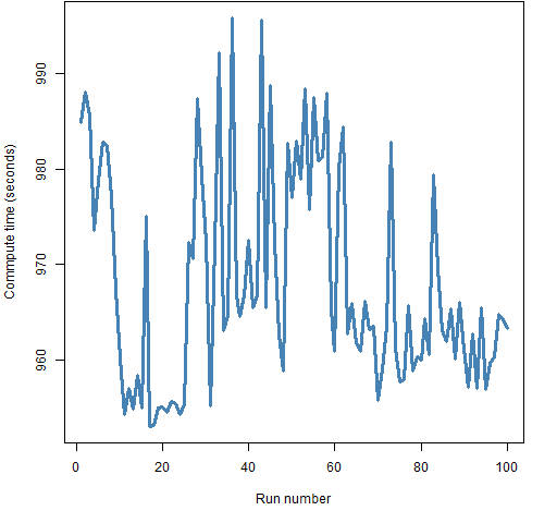
Besides, the timing (on Windows) seems dodgy. It is supposed to be timing only the compute time (not elapsed time), but the timings don’t seem to be following a constant plus noise model. Figure 1 shows an example of the timing.
Figure 1: The compute time reported for genopt in the order of the runs.  The timings are a bit suspect, but should be good enough.
The optimizers
Most of the optimizers used in “A comparison of some heuristic optimization methods” are also used here. The exception is the functions from NMOF because they don’t have explicit box constraints (there is a mechanism for imposing constraints though). The only unconstrained method that was run was the SANN method of the optim function.
Three methods were added.
pso package
The psoptim function from pso implements a particle swarm algorithm.
nloptr package
The Controlled Random Search (CRS) method was done via the nloptr function in the nloptr package.
This has the unexpected behavior of not respecting default values of arguments in the function to be optimized. You need to specify additional arguments to the function even when they have default values.
cmaes package
The Covariance Matrix Adapting Evolutionary Strategy is implemented in the cmaes package.
When the version from CRAN (1.0-11) was used on this problem, it got nowhere. The results presented here are from an R-forge version. Apparently the difference is the default values for control variables. Adjusting default values is a work in progress.
Results
Portfolio Probe consistently gets the same (best) answer in about 3 to 4 seconds.
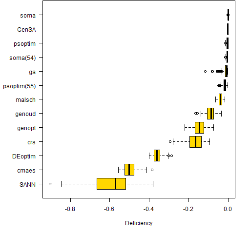
Figure 2 shows the distribution of deficiencies from the best answer for the methods.
Figure 2: Difference in utility from optimal (ordered by median).  The methods “soma(54)” and “psoptim(55)” are sets of runs where the time was significantly less than 1000 seconds. The number in parentheses is the mean time in seconds for the runs.
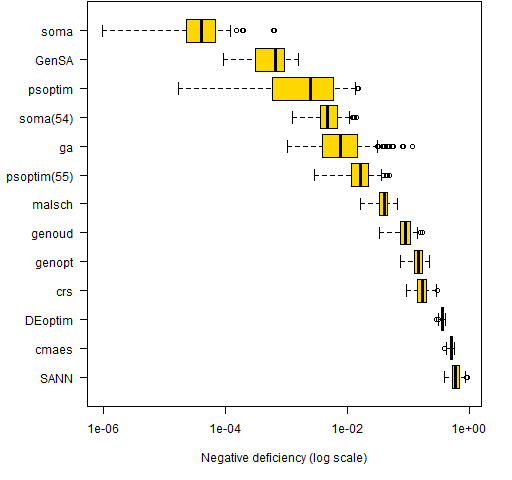
Figure 3 has the same information as Figure 2, but the sign of the numbers is changed and the plot is on the logarithmic scale.
Figure 3: Logarithm of negative difference in utility from optimal (ordered by median). 
Comments
Private correspondence with Enrico Schumann improved this section.
Defaults
This is not a comparison of algorithms. This is a comparison of algorithms with their mildly modified default values on one problem.
The importance of default parameters is evident with cmaes. The CRAN set didn’t even get out of the starting gate. The set that was used didn’t compare very favorably with the other optimizers. But it seems certain that there is a set of control parameters for it that would do very well.
Applications matter
The problem that is being solved has an effect on which algorithms (plus control parameters) work best. There is not a uniformly best algorithm.
Experimentation is useful
Experimenting with different algorithms and their settings is likely to pay off if you are doing the same sort of optimization repeatedly.
What is good enough?
There is almost always a point at which moving to a more optimal answer is not of practical relevance. That point will of course depend on the actual problem.
“What is good enough for portfolio optimization?” is an excellent question that I don’t think anyone has a good answer to. It does obviously depend on the quality of the inputs — if the inputs are complete garbage, then it doesn’t matter how close to optimal you are. (The correct answer in that case is not to trade at all.)
Clustering
Both soma and psoptim (and perhaps others) get relatively good answers within a minute, but then they never seal the deal, so to speak. They don’t get especially close to the best objective.
You may naively think that the longer runs would be scattered between where they are after a minute and the best solution.
Given:
- a problem
- an algorithm
- its control parameters
- the amount of time it runs
then there is an expected value for that random process. The Law of Large Numbers says that the actual result for any run is likely to be close to the expected value. That is the clustering we are seeing.
One star
There is one algorithm (besides Portfolio Probe) that has done well in all of the problems in this and the previous comparison: GenSA.
We don’t know how specific that is to the problems posed and its default parameters. But it seems worth keeping an eye on it.
Appendix R
The functions and data to reproduce this analysis are in heuristic_objs2.R (4 MB). The utility that Portfolio Probe achieves is -0.35776787228876. The non-zero optimal weights (to six decimal places) are in optimalWeightsAll.csv.
In case you want to test routines on these problems outside R: the variance is in varianceall.csv (4 MB) and the expected return vector is in expectedreturnsall.csv.

Just curious as to why time was used as you stopping criteria? I’ve done some work with a Matlab counterpart of a few of the above mentioned optimization algorithms, (PSO, GA, NLOpt package, and implicit filtering to name a few). Often we use some relative difference stopping tolerance, ie. stop when the previous x function values are within some small tolerance of each other. This method better guarantees convergence to the global optimum. We then proceed to use the number of function evaluations as a way to measure the algorithm’s efficiency. I find computer clocks can be a very unreliable tool, whereas the number of function evaluations is a more concrete value for measuring performance (averages can be taken for stochastic methods while deterministic algorithm’s will always require the same number of function evaluations given identical initial conditions). Also, using time provides no insight as to how certain algorithms might perform if they were operated in parallel. An explanation as to why time was chosen would be great!
Cheers,
Andrew
Andrew,
Thanks for your comments.
The two main reasons to use time were:
* people care about how long a computation takes
* using time was easy
Sometimes there is an explicit budget for time. Even if there isn’t, people are likely to have a limited tolerance for how long an optimization takes.
The number of function evaluations is quite a good measure to use. But I don’t think all of the optimizers have that as a stopping criterion (‘genopt’ does). However, there can be a problem with that if the function evaluations are very fast. In that case, some optimizers may be slower because they use a lot of time relative to the amount of time evaluating the objective function. (But that is also a problem for what I have done.)
In this comparison, I think using some sort of population convergence would not have been a good criterion. But if you have a real application that you care about, then you probably would want to use that. You could adjust control parameters for the algorithms you are testing so that they tend to converge within your time tolerance. Then pick the one that seems to be best in that setting.
I’m not convinced we can get much insight into how algorithms are likely to perform in a parallelized setting without doing the parallelization. How you parallelize an algorithm is sure to matter.
In summary, I think Andrew’s criticism is worth noting. Figuring out which optimizer will work best is hard.
Pingback: A comparison of some heuristic optimization methods | Portfolio Probe | Generate random portfolios. Fund management software by Burns Statistics