Much of what has been said and thought about beta in finance is untrue.
Myth 1: beta is about volatility
This myth is pervasive.
Beta is associated with the stock’s volatility but there is more involved. Beta is the ratio of the volatility of the stock to the volatility of the market times the correlation with the market.
A stock can be high beta by being volatile or by being highly correlated to the market.
Note that the correlation and volatilities are on returns not prices.
The math
If A is an asset and the market is M, then one way of writing beta of A is:
β = Cov(A, M) / Var(M) = Cor(A, M) * Vol(A) / Vol(M)
Well, actually that is two ways. “Cov” means covariance. “Var” means variance. “Cor” means correlation. “Vol” means volatility (annualized standard deviation).
Myth 2: beta is about risk
This one is actually true. But you have to read the fine print.
It is not risk as you are likely to think of it. Beta is an indication of the risk that can’t be diversified away by holding the market portfolio.
If you have an unnatural obsession with market portfolios, then this is a fine measure.
Myth 3: beta is well-estimated
Traditionally beta is estimated with 60 months of data. Let’s see how that does for IBM. (Since we are being traditional, the example has to be IBM.) Figure 1 shows the data.
Figure 1: Monthly returns for S&P 500 and IBM. The blue points are the most recent 60, black points are the previous 72.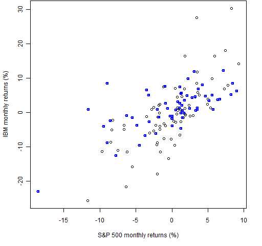 The regression for those latest 60 points gives us the coefficients:
> coef(lm(ibm.m60 ~ spx.m60))
(Intercept) spx.m60
0.01282182 0.74735429
So we get a beta of about 0.75 (and a positive alpha). We can see how variable beta is by doing a bootstrap:
> btm <- numeric(10000)
> for(i in 1:10000){
+ s60 <- sample(60, 60, replace=TRUE)
+ btm[i] <- coef(lm(ibm.m60[s60] ~ spx.m60[s60]))[2]
+ }
> plot(density(btm)) # basically Figure 2
> mean(btm > 1)
[1] 0.0459
> mean(btm < 0.5)
[1] 0.0966
So there is about a 4.5% chance that beta is more than 1 and almost a 10% chance that beta is less than 0.5.
Figure 2: Bootstrap distribution of IBM’s beta using 60 months of data.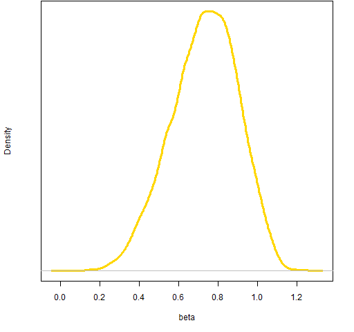
We don’t have to follow tradition and use 60 monthly data points. Let’s see what happens when we use 250 of the most recent daily returns.
> coef(lm(ibm.d250 ~ spx.d250))
(Intercept) spx.d250
0.0006039143 0.7440307042
> btd <- numeric(10000)
> for(i in 1:10000) {
+ s250 <- sample(250, 250, replace=TRUE)
+ btd[i] <- coef(lm(ibm.d250[s250] ~ spx.d250[s250]))[2]
+ }
> plot(density(btd)) # basically Figure 3
This gives almost exactly the same value as the monthly data (which is fairly accidental), and the estimate is much less variable. However, it is not as if it is free of variability.
Figure 3: Bootstrap distribution of IBM’s beta using 250 daily returns.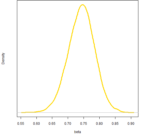
Myth 4: beta is stable
Many people think that a stock’s beta is a fixed value, as if it were tattoed on the stock’s forehead. I suspect that a beta that is stable through time is a very rare creature.
We can get a sense of the variability over time of IBM’s beta by looking at the two components of beta that we identified before:
- the ratio of the stock volatility to the market volatility
- the correlation between the stock and the market
We can get a reasonably good estimate of the ratio of volatilities on a daily basis by fitting a garch model to the daily S&P data and (separately) to the IBM data. The result of such an exercise is shown in Figure 4.
Figure 4: The ratio of daily IBM volatility to S&P 500 volatility as estimated by univariate garch models.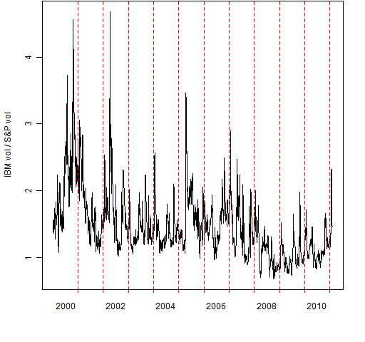
Getting instantaneous correlations is more problematic. But it is quite easy to get a 200-day rolling correlation, which is shown in Figure 5. The date of a correlation is the final day used in the calculation.
Figure 5: 200-day rolling correlation between IBM and S&P 500.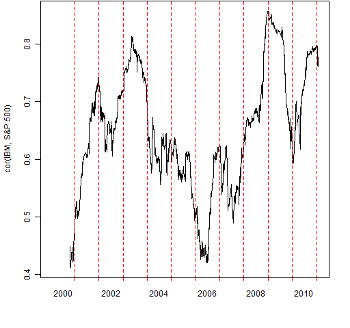
Finally, we can multiply the two components to get an estimate of beta over time. This is done in Figure 6.
Figure 6: Estimate of IBM’s beta through time.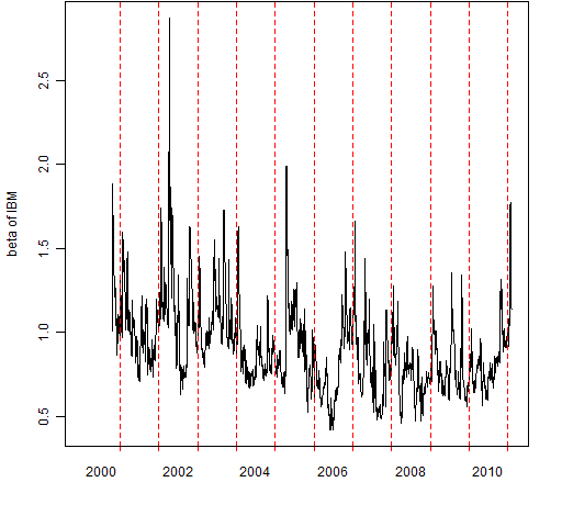
My guess is that if we had a daily estimate of correlation, then the estimate of beta would be even more variable.
Myth 5: beta comes from a sensible model
Beta comes from the Capital Asset Pricing Model (CAPM). This model says that the return of a stock is explained by the return of the market.
No one believes that the market is the only risk factor. Once upon a time it was expedient to make that assumption. These days we have data and computers — we don’t need to make that stupid assumption any more.
Now we have much more freedom in the stupid assumptions that we can make.
Broader context
So far we have only discussed beta as it pertains to a single stock, but the term “beta” has escaped CAPM into a broader context (as indeed has “alpha”).
In more general use “beta” means returns driven by exposure to risk. The statement:
That tech fund just gives you beta.
means that the speaker believes the fund only makes (or loses) money because of exposure to the technology market, as opposed to outperforming in a skillful manner (alpha). The beta that is implied is different than if the fund aimed at spanning the entire market.
On the internet
When I did an internet search on beta in finance, what I found tended to fall into two categories:
- nonsense
- something related to Wikipedia
The Wikipedia article on beta in finance is very good. Many of the sensible items in the first pages of the search use material from Wikipedia — some blatantly, some more subtly.
Questions
If you are doing an analysis and you think that beta is the answer, then you should ask yourself what the question is. Once you realize what the question is, then you should think about the best way to answer the question. My guess is that beta will seldom be the best approach.
Are there problems for which beta really is a useful statistic?
Updates:
- The post “Beta is not volatility” shows more about Myth 1
- The myth that a portfolio with beta equal 1 is like the index is busted in “The effect of beta equal 1”
Appendix R
The analysis and plots were done with R. The script of the R commands for the analyses in this post is beta_myth.Rscript
Update: Josh Ulrich got a couple errors from the script above, so he kindly sent a revised script that works for him, and it also shows a simplified way of getting the running correlation. It is beta_myth_jmu.Rscript
To get the pp.timeplot function that was used for Figures 4, 5 and 6 into your R session, you can do the command:
> source('https://www.portfolioprobe.com/R/blog/pp.timeplot.R')
Pingback: Wednesday links: articulate confabulators Abnormal Returns
Good post although none of the analysts I know that are evaluated on security analysis including myself utilize beta. I strongly suspect that the perception of the usefulness of beta and the CAPM is perpetuated by analysts and portfolio managers that are not held accountable for security analysis such as sell side analysts, financial advisors, wealth management shops, and anyone looking to appear to have some analysis behind a recommendation. Most importantly, beta is an easy way to justify your cost of capital for project financing without opening yourself up to criticism from someone looking to promote or sink the project.
Stephen,
Thanks for the comment. I’m guessing that there is a lot of inertia involved — people used to do it, so we feel compelled to continue. Doing what has always been done is much easier than thinking about what should be done.
Pingback: Tweets that mention 4 and a half myths about beta in finance | Portfolio Probe | Generate random portfolios. Fund management software by Burns Statistics -- Topsy.com
Pingback: Quora
What would you recommend to use if, for example, you wanted to find the optimal way to hedge a given stock position against market movement? I gather you are not a fan of beta; but are you saying there is no way to hedge anything?
Pingback: Anonymous
The change in beta might be influenced by the capital structure.
Imo, if you dont want market risk, dont be in the market
Pingback: Beta is not volatility | Portfolio Probe | Generate random portfolios. Fund management software by Burns Statistics
Pingback: Low (and high) volatility strategy effects | Portfolio Probe | Generate random portfolios. Fund management software by Burns Statistics
Pingback: Blog year 2011 in review | Portfolio Probe | Generate random portfolios. Fund management software by Burns Statistics
Pingback: On smart beta | Portfolio Probe | Generate random portfolios. Fund management software by Burns Statistics