Some facts and some speculation.
Definition
Volatility is the annualized standard deviation of returns — it is often expressed in percent.
A volatility of 20 means that there is about a one-third probability that an asset’s price a year from now will have fallen or risen by more than 20% from its present value.
In R the computation, given a series of daily prices, looks like:
sqrt(252) * sd(diff(log(priceSeriesDaily))) * 100
Usually — as here — log returns are used (though it is unlikely to make much difference).
Historical estimation
What frequency of returns should be used when estimating volatility? The main choices are daily, weekly and monthly. (In some circumstances the choices might be something like 1-minute, 5-minute, 10-minute, 15-minute.)
There is folklore that it is better to use monthly data than daily data because daily data is more noisy. But noise is what we want to measure — daily data produces less variable estimates of volatility.
However, this is finance, so things aren’t that easy. There is the phenomenon of variance compression — that is, it isn’t clear that volatility from monthly and daily data are aiming at the same target.
Another complication is if there are assets from around the globe. In that case asynchrony is a problem with daily data. For example, the daily return of assets traded in Tokyo, Frankfurt and New York for January 21 are returns over three different time periods. That matters (not much for volatility, but definitely for correlations). Weekly returns as well as fancy estimation methods alleviate the problem.
Through time
Volatility would be more boring if finance were like other fields where standard deviations never change.
Financial markets seem to universally experience volatility clustering. Meaning that there are time periods of high volatility and periods of (relatively) low volatility.
But why?
Changes in volatility would make sense if there were periods of greater uncertainty about the future. But the future is always uncertain.
The day after Lehman Brothers failed there was a great deal more uncertainty about the markets than the week before. However, that uncertainty was generated internally to the markets, it wasn’t greater uncertainty about the physical world.
Agent-based models of markets easily reproduce volatility clustering. Rather than agents changing their minds about the best strategy at random times, mind-changing tends to cluster. When lots of agents change strategies, then the market volatility goes up.
Across assets
Different assets in the same market have different volatilities. But why?
Some assets are especially responsive to the behavior of the rest of the market. Some assets are inherently more uncertain.
Factor models explicitly divide these two ideas into systematic and idiosyncratic risk.
Implied volatility
Implied estimates come from using a model backwards. Suppose you have a model that approximates X by using variables A, B and C. If you know X, A and B, then you can get an implied estimate of C by plugging X, A and B into the model.
An example is implied alpha.
Implied volatility comes from options pricing models. The most famous of these is the Black-Scholes formula.
Black-Sholes uses some assumptions and derives a formula to say what the price of an option should be. The items in the formula are all known except for the average volatility between the present and the expiration date of the option.
We can use known options prices and the Black-Scholes formula to figure out what volatility is implied. You can think of this as the market prediction of volatility — assuming the model is correct (but it isn’t).
Not risk
Some people equate volatility with risk. Volatility is not risk.
Volatility is one measure of risk. In some situations it is a pretty good measure of risk. But always with risk there are some things that we can measure and some things that escape our measurement.
Part of risk measurement should be trying to assess what is left outside.
Epilogue
Before I built a wall I’d ask to know
What I was walling in or walling out,
And to whom I was like to give offense.
from “Mending Wall” by Robert Frost
Appendix R
I made the statement that using simple returns rather than log returns is unlikely to make much difference. We shouldn’t take my word for it. We can experiment.
In most blog posts I give only a sample of the R code. Here, though, is the complete R code for this experiment.
write a function
pp.dualvol <- function(x, frequency=252) {
   lv <- sd(x)
   sv <- sd(exp(x)) # same as sd(exp(x) - 1)
   100 * sqrt(frequency) *
      c(logReturn=lv, simpleReturn=sv)
}
get starting points of the samples
starts <- sample(length(spxret) - 253, 1000)
This statement presumes that the number sampled is smaller than the number of values being sampled since it is using the default of sampling without replacement.
compute volatilities
volpairs <- array(NA, c(1000, 2),
   list(NULL, names(pp.dualvol(tail(spxret, 10)))))

tseq <- 0:62

for(i in seq_along(starts)) {
   volpairs[i,] <- pp.dualvol(spxret[starts[i] + tseq])
}
write plot function
P.dailyVolPair63 <-
 function (filename = "dailyVolPair63.png")
 {
    if(length(filename)) {
       png(file=filename, width=512)
       par(mar=c(5,4, 0, 2) + .1)
    }
    plot(volpairs, col="steelblue")
    abline(0, 1, col="gold")
    if(length(filename)) {
       dev.off()
    }
 }
do the plot
P.dailyVolPair63()
Figure 1: Volatility estimates on a quarter of daily data — simple versus log returns. 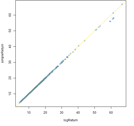
We can see that almost all of the 1000 estimates are virtually the same when using either type of return. There are a few large volatilities that are slightly different. The differences will be due to large returns, which means that returns at lower frequencies will yield bigger differences between the volatility estimates.

Your comment “You can think of this as the market prediction of volatility — assuming the model is correct (but it isn’t).” is factually incorrect.
Backing out implied volatilities from quoted options prices gives you the EXACT market implied volatilites, the expected volatility of future returns that the market expects. The market applies certain coventions andwhile the Black Scholes model itself makes incorrect assumptions about return distributions and an number other issues, for example equity market participants ALL relate option prices to the underlying volatility through Black Scholes, hence assuming one uses the same “translation tool” as the market does one can derive the specific market implied volatilities from option prices and those are entirely model assumption independent!
Matt,
Yes, my statement wasn’t quite coherent.
It seems to me that you are saying that if everyone looks through the same distorting glasses, then they will agree on the description of the world.
I was emphasizing that models are distorting glasses. I failed to mention that people don varying distorting glasses, which is how the ambiguity of “market view” arises.
A very interesting article.
Pingback: » Note from 1/20/1014 to …MarkR
Pingback: If you did not already know: “Volatility” | Data Analytics & R