How did the constraints affect portfolio betas, and how did the betas change over time?

Previously

“Low (and high) volatility strategy effects” created 6 sets of random portfolios — the so-called low vol cohorts — as of 2007 and showed their performance up to about a month ago.

“Rebalancing the low vol cohorts” looked at how much turnover was required to move back to the constraints.

“Maximum weight of the low vol cohorts” examined how the maximum weight drifted through time.

“Beta is not volatility” showed that beta and volatility are distinct concepts.

This post looks at the portfolio betas of the six sets of portfolios.

Pictures

There are three distributions in each plot:

• gold: the initial portfolios at the initial time
• blue: the initial portfolios at the final time
• black: the rebalanced portfolios at the final time

Figure 1: Distribution of portfolio beta for the “vanilla” portfolios. 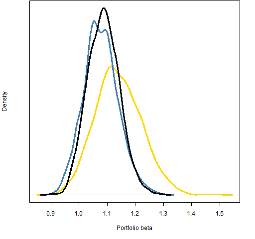For the “vanilla” portfolios the beta drifts slightly lower and becomes a little more concentrated.  The rebalancing hardly affects beta at all except for slightly pulling in the tails.

Figure 2: Distribution of portfolio beta for the “low variance” portfolios. 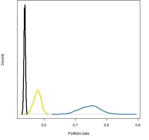For the “low variance” portfolios beta drifts significantly higher and disperses.  The rebalancing then pulls beta into a tight range that is lower than the original.

Figure 3: Distribution of portfolio beta for the “low volatility” portfolios.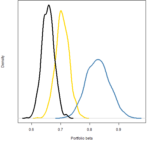

Figure 4: Distribution of portfolio beta for the “low beta” portfolios. 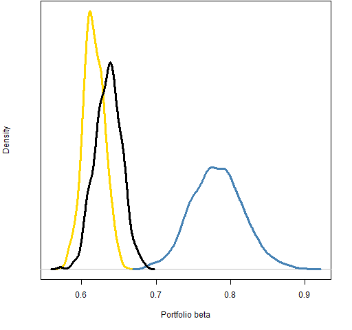Notice that the initial distribution for the “low variance” portfolios is lower than the initial distribution of the “low beta” portfolios.  That’s an indication that the constraint to get “low beta” is not particularly vigorous.

Figure 5: Distribution of portfolio beta for the “high volatility” portfolios.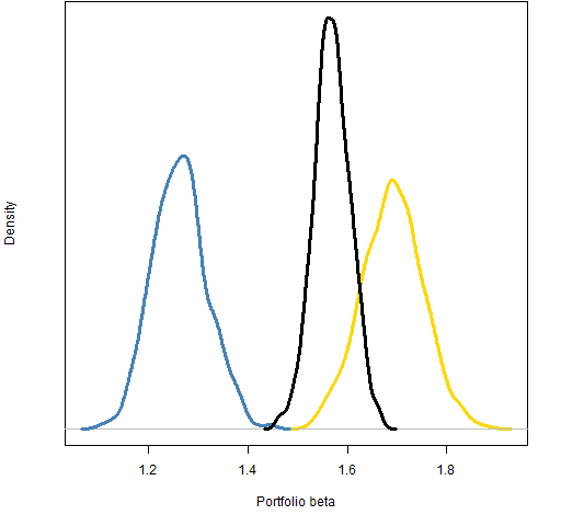
Figure 6: Distribution of portfolio beta for the “high beta” portfolios.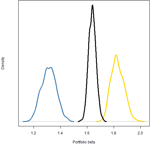

Fresh portfolios

The black distributions are different from the gold distributions.  Two possible reasons for this are:

• the shape of the market has changed
• the portfolios are generated at a previous time and then rebalanced

We can distinguish between these possibilities by generating fresh random portfolios at the final point.  Figures 7 and 8 show two examples — the green distribution is from the portfolios generated directly at the final time.

Figure 7: Distribution of portfolio beta at the final time for the “low variance” portfolios.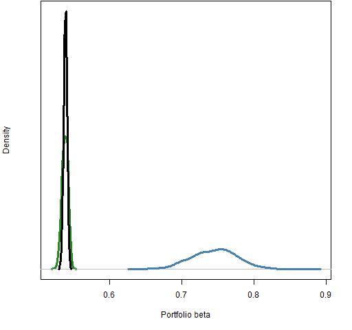

Figure 8: Distribution of portfolio beta at the final time for the “high beta” portfolios.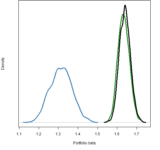

Figures 7 and 8 certainly favor the first hypothesis that the market changes.

Summary

• The beta distributions are quite distinct in the “low variance” cohort — probably since there is some optimization happening and not just selection.
• The nature of beta seems to be different at the two time points.

Appendix R

Two R functions were written for this post:

• pp.randportbeta takes a random portfolio object, a price vector and a vector of asset betas; it returns a vector of the portfolio betas.  The definition is in pp.randportbeta.R
• pp.tripleden takes three numeric vectors and plots their densities.  The definition is in pp.tripleden.R

Subscribe to the Portfolio Probe blog by Email