How wide is the darkness?

Uses of models

The main way models are used is to:

• shine light on the “truth”

We create and use a model to learn how some part of the world works.

But there is a another use of models that is unfortunately rare — a use that should be common in finance. That use is to:

• measure the darkness

We can use models to see how much we don’t know.

Incredible darkness of being

With the statistical bootstrap and simulation, it is very easy to use models to see the extent of our ignorance.  So why are models not used this way more?  I think it is because we want to maintain the illusion that we know what we are doing.

People want to believe their models are true.  It is perfectly possible to explore how much you don’t know by using a model that you fully believe.  But the psychology of believing in a model is not so much to have something to believe in as to deny ignorance.

mathbabe in a recent post suggests that macroeconomics could use a dose of ignorance as well.

Stock returns

Let’s use the return of the S&P 500 during 2011 as an example of discovering our ignorance.

We think we know the answer exactly — the index returned zero in 2011 (to the nearest basis point). But markets are random things.  If some people happened to have made different choices, the result for the year would have been different.  We can use models to see what sort of differences are likely.

The first thing we can do is bootstrap the daily returns during the year.  This suggests — as Figure 1 shows — that we are vastly ignorant about the return of the index.

Figure 1: Distribution of 2011 S&P 500 log return based on bootstrapping daily log returns, with 95% confidence interval.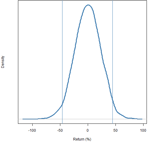

The 95% confidence interval based on bootstrapping the daily returns runs from about -46% to 45%.  Comparing this distribution to the actual distribution of yearly returns from 1950 through 2010 (Figure 2), we conclude that the daily bootstrap distribution suggests essentially total ignorance.

Figure 2: Distribution of S&P 500 annual log returns from 1950 through 2010. 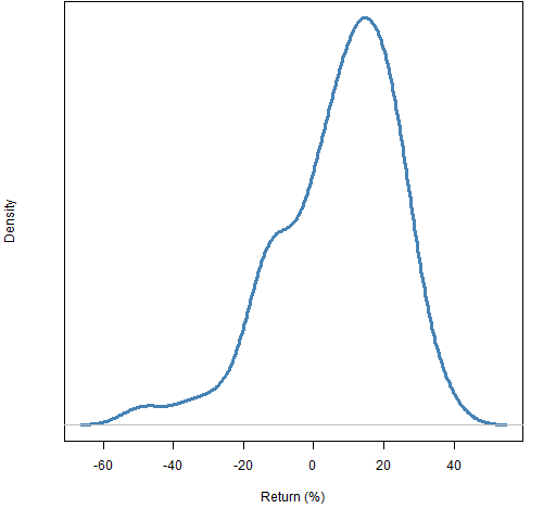But what is wrong with the model we’ve used?  It assumes (almost) that daily returns are independent and identically distributed.  That isn’t true.  Certainly there is volatility clustering, and probably some sort of autocorrelation.  Let’s try a different model.

Instead of using daily returns we can use overlapping 21-day returns.  This reduces the severity of the assumptions that we are making.  Figure 3 shows this alternative bootstrap distribution.

Figure 3: Distribution of 2011 S&P 500 log return based on bootstrapping overlapping 21-day log returns, with 95% confidence intervals: monthly (gold) and daily (blue). 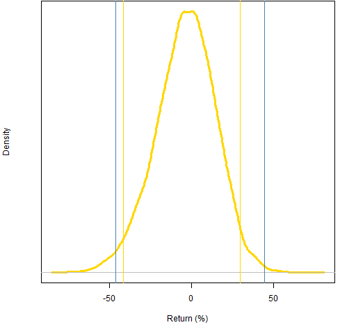That the monthly returns produce a narrower confidence interval than the daily returns is connected to the phenomenon of variance compression. (However, the confidence interval is quite variable when this procedure is done with permutations of the daily returns, so not too much faith should be put on the location of the gold lines.)

We can steal the idea used in the posts on yearly predictions and create a model purpose-built to make the unknown as small as possible.  Instead of using returns we use the residuals from an overly volatile model of the mean return.  We then need to bootstrap with blocks because these residuals are most certainly autocorrelated.

Figure 4 shows the loess fit that is used.  One day in August the expected value of the daily return was about -4% and a week later it was about +1%.  This model is sucking up a lot of variability.

Figure 4: The loess fit of daily S&P 500 returns through 2011. 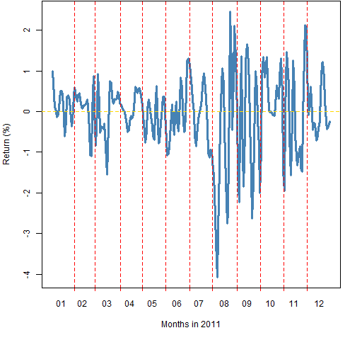This is a model intended not to be believable.  It is meant to be less smooth than the true expected value process of the returns.  If the index had followed this path, it would have lost about 14.7%.  We use the residuals from this fit to bootstrap.

Figure 5: Distribution of 2011 S&P 500 log return based on bootstrapping loess residuals, with 95% confidence intervals: loess (black), monthly (gold) and daily (blue). 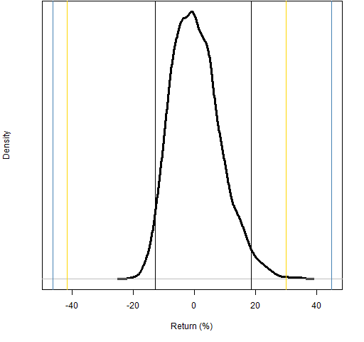The new confidence interval runs from about -13% to 18%. Notice that things are a bit strange in that the “center” (-14.7%) is outside the confidence interval.

We still have a wide interval after trying to squeeze out as much noise as possible.

Questions

What other models might be used to get the return distribution?

How rough is the actual expected value of returns?

How well did Google do at translating the two lines below?

Epilogue

Preguntale al polvo de donde nacimos.
Preguntale al bosque que con la lluvia crecimos.

Ask the dust from which we were born.
Ask the rain forest that grew.

from “Soy Luz y Sombra” (I am Light and Shadow)

Appendix R

As per usual, the computations were done in R.

simple bootstrapping

Bootstrapping the daily returns is a trivial exercise with three steps (create the object to hold the answer, fill the object with values, plot it):

spx_dboot <- numeric(1e4)
for(i in 1:1e4) spx_dboot[i] <- sum(sample(spx_ret2011, 252, replace=TRUE))

plot(density(spx_dboot))

block bootstrapping

Bootstrapping the overlapping monthly data is slightly more involved.

It was useful first to define a function that creates the overlapping returns:

pp.overlappingsum <-
function (x, n)
{
  cx <- c(0, cumsum(x))
  tail(cx, -n) - head(cx, -n)
}

This uses a couple tricks.  The idea of the function is to  get the sum of each set of consecutive sums with the difference of the cumulative sums at the two ends of the periods.

It also uses negative values for the second argument of head and tail.  This says get the head or tail of the vector except for some number of elements.

tail(x, 5)

says give me the last 5 elements of x.

tail(x, -5)

says give me all but the first 5 elements of x.  If x has length 10, then those are equivalent.

Now we use the function:

spx21ret_2011 <- pp.overlappingsum(spx_ret2011, 21)

There is the possibility that our tricky function would build up errors, but checking the last value against doing the sum directly yielded precisely the same answer.

The bootstrapping itself is back to mundane:

spx_mboot <- numeric(1e4)
for(i in 1:1e4) spx_mboot[i] <- sum(sample(spx21ret_2011, 12, replace=TRUE))

loess

We fit a loess model with a very small span:

spx11.loe <- loess(y ~ x, data=data.frame(y=spx_ret2011, x=1:252), span=7/253)

The names don’t appear on the fit the way we created the data, so we do it now since pp.timeplot requires names:

spx11_loefit <- fitted(spx11.loe)
names(spx11_loefit) <- names(spx_ret2011)
pp.timeplot(spx11_loefit, div='month')

We create the vector of residual blocks to bootstrap with:

spx11.lor21 <- pp.overlappingsum(resid(spx11.loe), 21)

By the way, this bootstrap distribution is quite insensitive to the length of the blocks.

 

Subscribe to the Portfolio Probe blog by Email