If a particular prediction comes true, how surprised should we be?
The prediction
The page that sparked my curiosity tells of a prediction made a year ago that the S&P 500 would beat its historic high by the end of 2011. It says that at the point the prediction was made, the level of the index was about 1010.
According to Wikipedia the all-time high close was 1565.15 on 2007 October 09, and the all-time intraday high was 1576.09 on 2007 October 11.
The surprise
So if the prediction actually comes to pass, then how surprised should we be?
To answer that let’s do a simulation using randomly selected daily log returns from the S&P 500. We want to see — over that year and a half period — the probability of the high being higher than the historical high. We can see an estimate of that probability using an R function written for the purpose:
> spx.predtest1()
[1] 0.048493
> spx.predtest1()
[1] 0.048307
So almost a 5% chance of getting a new all-time high. That is done with the data I happened to have hanging about. It starts in 1950.
We can instead use only more recent data. Here is a go with about a decade of data:
> spx.predtest1(rets=tail(spxret, 2500))
[1] 0.063795
> spx.predtest1(rets=tail(spxret, 2500))
[1] 0.064094
This gives on the order of a 6.4% chance of getting a new high.
But wait
I’ve lied to you up until now. Actually there was a get-out-of-jail condition on the prediction. It said:
“If the Index held at or above our proprietary support zone (1000.00- 950.00 region), it would eventually trade to a new historical high within 12 – 18 months (July- December 2011 timeframe)”
So instead of accepting all paths, we need to throw out paths that take us below 950 unless a new high happens first. It’s not hard to write an R function for that:
> spx.predtest2()
[1] 0.1009603
> spx.predtest2()
[1] 0.09969513
With the full set of returns the probability of this scenario is just about 10%.
> spx.predtest2(rets=tail(spxret, 2500))
[1] 0.2560359
> spx.predtest2(rets=tail(spxret, 2500))
[1] 0.2607624
The probability increases to over 25% with a decade of data.
And now
Fair enough for someone to remind the public of their predictions. But perhaps there is selection bias in the reminders (I have no idea if this particular prognosticator has such bias or not).
If we were completely sceptical, then we would take this as a new prediction from now until the end of the year. If we skip the complication of the conditional, we can look at the probability of the S&P hitting an all-time high in the approximately 125 trading days from the beginning of July until the end of the year:
> spx.predtest1(target=log(1577/1320.64), time=125)
[1] 0.141888
> spx.predtest1(target=log(1577/1320.64), time=125)
[1] 0.141285
We get a chance of about 14%.
> spx.predtest1(target=log(1577/1320.64), time=125, rets=tail(spxret, 2500))
[1] 0.197302
> spx.predtest1(target=log(1577/1320.64), time=125, rets=tail(spxret, 2500))
[1] 0.197462
With the returns restricted to the last decade we get almost 20%.
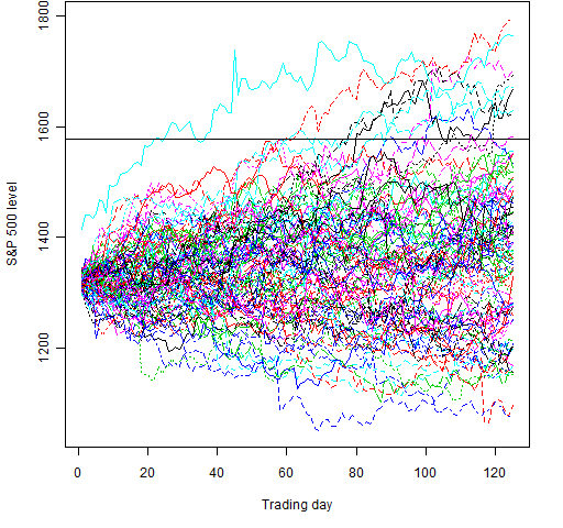
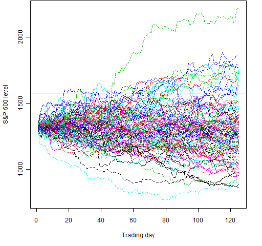
Figures 1 and 2 each show 100 random paths for these cases.
Figure 1: 100 random paths for July through December in 2011 using 6 decades of data. 
Figure 2: 100 random paths for July through December in 2011 using the most recent decade of data.
Analysis weaknesses
We get substantially different answers depending on if we use one or six decades of data. That is because volatility changes over time. A better approach would be to use a garch model to simulate the returns where the simulation starts with the volatility state of July 2010 (or July 2011 for the last analysis).
Appendix R
Except for the axis labels, the two figures were made by:
> rmat6 <- matrix(sample(spxret, 12500, replace=TRUE), nrow=125)
> lmat6 <- 1320.64 * exp(apply(rmat6, 2, cumsum))
> matplot(lmat6, type='l')
> abline(h=1577)
>
> rmat1 <- matrix(sample(tail(spxret, 2500), 12500, replace=TRUE), nrow=125)
> lmat1 <- 1320.64 * exp(apply(rmat1, 2, cumsum))
> matplot(lmat1, type='l')
> abline(h=1577)
The definition of spx.predtest1 is:
function (rets=spxret, target=log(1577/1010), time=370, trials=1e6)
{
hits <- 0
for(i in 1:trials) {
this.ret <- max(cumsum(sample(rets, time, replace=TRUE)))
if(this.ret > target) hits <- hits + 1
}
hits/trials
}
The definition of spx.predtest2 is:
function (rets=spxret, target=log(1577/1010), low=log(950/1010), time=370, trials=1e5)
{
hits <- 0
allowed <- 0
both <- 0
for(i in 1:trials) {
this.ret <- cumsum(sample(rets, time, replace=TRUE))
retran <- range(this.ret)
if(retran[1] > low) {
allowed <- allowed + 1
if(retran[2] > target) hits <- hits + 1
} else if(retran[2] > target) {
both <- both + 1
# is high before low?
if(min(which(this.ret > target)) < min(which(this.ret < low))) {
allowed <- allowed + 1
hits <- hits + 1
}
}
}
# c(hits=hits, allowed=allowed, both=both, prob=hits / allowed)
hits / allowed
}

Hello dear Pat,
Might you consider using
library(colorspace)
rainbow_hcl
For the next time you make such a plot?
🙂
Cheers,
Tal
Tal,
Thanks — I’ll have a play some time.