Are there times of the year when returns are better or worse?
Abnormal Returns prompted this question with “SAD and the Halloween indicator” in which it is claimed that the US market tends to outperform from about Halloween until April.
Data
The data consisted of 15,548 daily returns of the S&P 500 starting in 1950. Then the point along the year was found for each day.
Method
The lowess smoother was used to find the typical return for each point in the year. To see how surprising the deviations are, 1000 instances of permuting the returns (so that there is no trend) were smoothed in the same manner.
Results
Figure 1 shows the smoothing using the default settings. As with all the plots, the smooths of the 1000 permuted datasets are shown in thin gold lines, and the smooth of the actual data is shown with a thick blue line.
Figure 1: Lowess smooth with span=2/3 on the full data.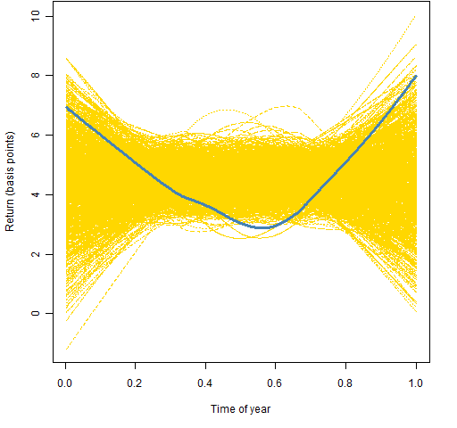 Figure 1 is suggestive that the summer has lower returns — consistent with Halloween indicator theory. However, this is really over-smoothed. Figure 2 uses a more reasonable level of smoothing.
Figure 2: Lowess smooth with span=0.1 on the full data. 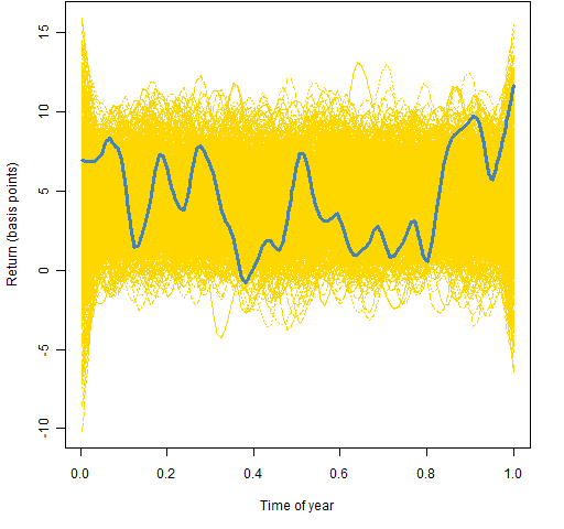 With this level of smoothing there appears to be a possibility of a brief bad time in the second quarter, and possibly high values in the fourth quarter. We can investigate further by breaking the data into two parts — shown in Figures 3 and 4.
Figure 3: Lowess smooth with span=0.1 on the data from 1950 through 1979. 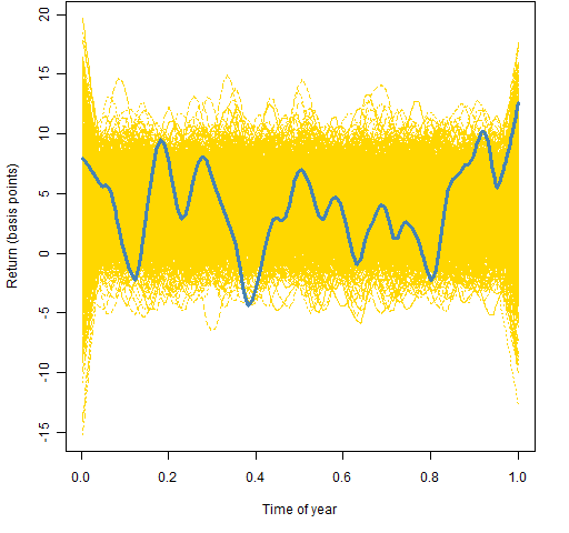
Figure 4: Lowess smooth with span=0.1 on the data from 1980 to the present. 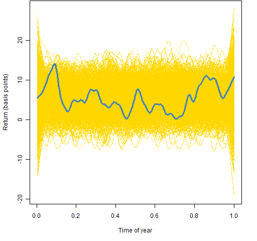 Figure 4 exhibits the pattern suggested by the Halloween indicator but nowhere near to an extent that should surprise us. Figure 5 checks to see if the pattern has strengthened lately.
Figure 5: Lowess smooth with span=0.1 on the data from 2000 to the present. 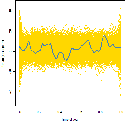 The smooth looks to be flatter in this century.
Summary
The answer to the question in the title seems to be: Probably not.
There have to be periods from the data that are higher than others. However, to believe that there is a real pattern we should demand that what we observe looks different than random data. The real data and random data are quite similar in this instance.
Questions
lowess is handy, but it isn’t really doing the smoothing that we want. In this case 0 and 1 are the same — we really want to do circular smoothing so that the ends of the year are tied together. What are the best choices in R for circular smoothing on this sort of data?
Not a qeustion, but: The plots exhibit a known weakness of lowess in that the ends are very variable — going off in straight lines. lowess should never be used to extrapolate outside the data range.
Appendix R
data update
I already had a vector of S&P 500 returns starting in 1950. To update that, I did:
require(TTR)
spxnew <- getYahooData('^GSPC', 20100601, 20111017)
spxnewret <- drop(as.matrix(diff(log(spxnew[, 'Close']))))[-1]
The next step was to check that the overlap matched. Good practice when updating data — especially automatic updates — is to have an overlap and check equality of the overlap.
Then, of course, the two were put together:
spxret <- c(spxret, spxnewret[-1:-21])
time of year
Now create the fraction along the year for each day.
spxyears <- substring(names(spxret), 1, 4)
spxyrtab <- table(spxyears)
sp.tlist <- lapply(spxyrtab, function(x) seq(to=x))
spxyrtab[62] <- 252 # current year is only partial
sp.tlist2 <- mapply(`/`, sp.tlist, spxyrtab)
spxseason <- unlist(sp.tlist2)
If you were doing this a lot so that computational time mattered, then there is undoubtedly a clever way of doing this with the data.table package.
smoothing and permuting
spx.low <- lowess(spxret ~ spxseason)
lowperm.ymat <- array(NA, c(15548, 1000))
for(i in 1:1000) lowperm.ymat[,i] <- lowess(spxret ~ sample(spxseason))$y
plotting
Figure 1 was created by:
plot(spx.low$x, spx.low$y*1e4, xlab="Time of year", ylab="Return (basis points)", type="n", ylim=1e4 * range(spx.low$y, lowperm.ymat))
matlines(spx.low$x, 1e4*lowperm.ymat, col="gold")
lines(spx.low$x, spx.low$y*1e4, lwd=3, col="steelblue")
Pingback: Thursday links: justify your fees | Abnormal Returns
David Merkel suggested the addition of p-values. These can be easily found using minimal assumptions via a permutation test.
Here are some (based on 10,000 permutations):
1950 – present: less than .001
1950 – 1979: less than .001
1980 – present: .02
2000 – present: .12
P-values may please those schooled in frequentist statistics, but they aren’t necessarily easy to interpret.
The very small p-value for the early period may be selection bias — that the indicator is alive because of the data we are basing the test on. Wikipedia says that it is a feature of markets in several countries, so the selection argument has less weight in that light.
The higher p-value for the 2000-to-present period could be because it is based on fewer datapoints. Using non-overlapping periods of the same length (2967), we get p-values of: .03, .03, .05, .08.
This analysis makes me want to change my conclusion. I’m inherently skeptical of such things, but it looks like the effect actually may have been real. However, it seems to be fading away.
Well done. I agree with your tentative conclusions.
The permuted data in figure 1 appear very different from that in the later plots. So comparing loess span size is apples and oranges, or am I missing something?
Michael,
I’m confused about where you are confused.
In all plots the same span is used for the actual data and the permutations. Figure 1 is different than the rest in that it uses a much larger span than the others.