Investors need to distinguish between good and bad active fund managers.  Relatively new technology makes this much easier.

The usual methods

benchmark

One of the common approaches is to compare funds versus a benchmark.  Often much effort goes into choosing just the right index to be the benchmark.  Should we use MSCI or something else?  But no matter which index you select, the test will be anemic.

Suppose:

• you have 10 years of quarterly data
• you have a 5% chance of accepting a fund with no skill at all
• you are looking for funds with an information ratio of one-half

Then you will accept less than half of the skilled funds.  If no-skill funds are much more common than skilled funds, the non-skilled funds may dominate.

This analysis is making favorable assumptions — the reality is that the test is much worse.  The issue is that the difficulty of outperforming the benchmark varies over time.  I’m not sure how to parameterize that, but I’m guessing we’d be talking two or three decades (at least) instead of one.  And how many funds will have constant skill for decades?

peer group

The other common approach is to use peer groups: how good is the fund relative to similar funds?  That’s a logical question to ask, but we probably won’t get a very good answer by using peer groups.

A key assumption is that the ranking of the returns within the group has more to do with skill than luck.  That assumption is probably false.

A better method

We can randomly generate portfolios that obey the constraints of the fund in question.  Then compare — over some time period — the return of the fund to the distribution of returns of the random portfolios.

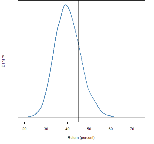
Figure 1 is an example.  The fund performed above the average, but not well enough to believe it was anything but luck.  This is the technique advocated by Ron Surz (and others).  Ron has an implementation of it called Portfolio Opportunity Distributions (PODs).

Figure 1: Fund return relative to distribution of static random portfolios.

The technique is reminiscent of peer groups, but here the “peers” are portfolios that the fund might have held.  There is no need to compromise on the number of them, or on how closely they resemble what the fund does.  Unlike with peer groups, we know what the comparison with the distribution means because we know the skill of all the “peers” in the distribution (zero skill).

This is better, but not especially good.  One problem is that the distribution is wide — we see what luck looks like, but it encompasses a lot.  In order to see something as skill, it might have to be exceptional skill.

Better still

We can get narrower distributions (sometimes much narrower) by using additional information:

• the positions of the fund at the start of the time period
• the turnover throughout the time period

The trick is to create a number of paths over the time period.  Each path starts with the same positions as the actual fund, but then random trading is done throughout the time period.  The random trades obey both the constraints of the fund and the turnover for the fund.  The returns of the paths for the time period are then found.  This is called the shadowing method.

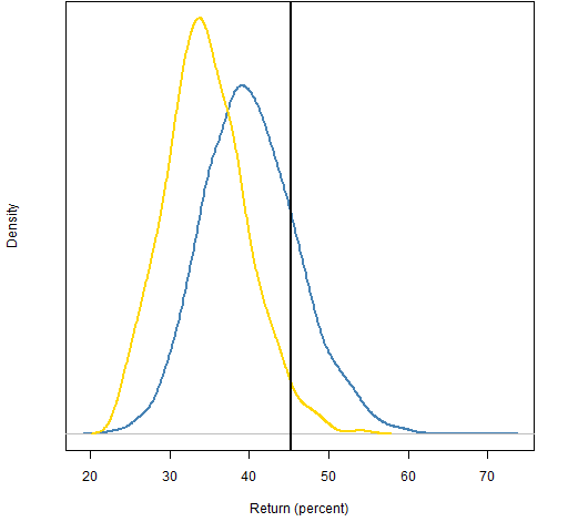
Figure 2 shows both distributions in a case where there is 200% turnover (buys plus sells) over a year.

Figure 2: Fund return relative to the static distribution (blue line) and the shadowing distribution (gold line).  The assessment of skill is much different in this case from the two methods.  The fund return is far enough into the tail of the shadowing distribution that we might consider the possibility of skill (about 3% in the tail).  If the return had been on the order of 25% to 30%, then the static distribution would indicate negative skill while there would be no surprise with the shadowing distribution.

The initial portfolio of the fund could be anywhere in the static distribution.  The shadowing method eliminates the bias that the static method has of implicitly assuming that the intial portfolio is at the center of the static distribution.

Performance should be measuring the effect of decisions that fund managers make.

Getting it done

Investors interested in particular funds could gather data together and do the analyses.  However, it is more sensible for fund managers to do the analyses themselves.  The reasons include:

• the analysis is done once rather than many times
• all the pertinent data are readily available
• it will be educational for the fund manager

To expand on the last point, the act of performing the random portfolio analysis is likely to improve the investment process of the fund manager.  They will be better able to see what works and what doesn’t work in their process.

It is in investors’ interests to encourage fund managers to use random portfolios for performance measurement and then to make the analyses available to investors.  The result will be much more clarity regarding the skill of fund managers, easing the task of selecting managers.

Example details

The data are almost all of the constituents of the S&P 500.  The year was 2009.  The fund maximizes the return where the expected returns are given by an MACD computation (a momentum strategy).

The constraints were 90 to 100 assets in the portfolio, and a maximum weight of 10%.  The 200% turnover was divided equally among the 13 rebalances that occurred every 20 trading days.

A real case would almost surely use a variance matrix and maximize the information ratio or a mean-variance utility.  I was being lazy and didn’t create an appropriate set of variance matrices.

Subscribe to the Portfolio Probe blog by Email