If returns had infinite variance, would there be a problem bootstrapping information ratios?
Background
There is a discussion on the Quant Finance group of LinkedIn with the title: “How do you measure the confidence intervals of performance ratios?”
One suggestion was to use the statistical bootstrap. This resulted in a discussion of the efficacy of the bootstrap under infinite variance. There is actually a missed step in there — just because the returns have infinite variance doesn’t mean that the performance ratios will. This post looks at the distribution of the information ratio under a few distributions of returns including some with infinite variance.
I don’t believe that returns do have infinite variance, but we’re considering consequences if they did.
By the way, my answer to the broader question of how to determine if a fund outperforms is to use random portfolios.
Simulations
Returns were simulated and the information ratio for the returns was computed. The number of returns used was either 12 (as in a year of monthly data) or 60 (as in a quarter of daily data). The distribution of the information ratios is plotted using a normal qqplot. The lines in the plots show the behavior of the extreme quartiles relative to the middle quartiles.
Figures 1 and 2 are for normally distributed returns. If — as in these plots — the points are essentially on a line, then the distribution is normal.
Figure 1: QQplot using 12 normally distributed returns. 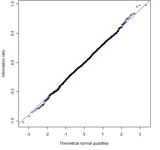
Figure 2: QQplot using 60 normally distributed returns.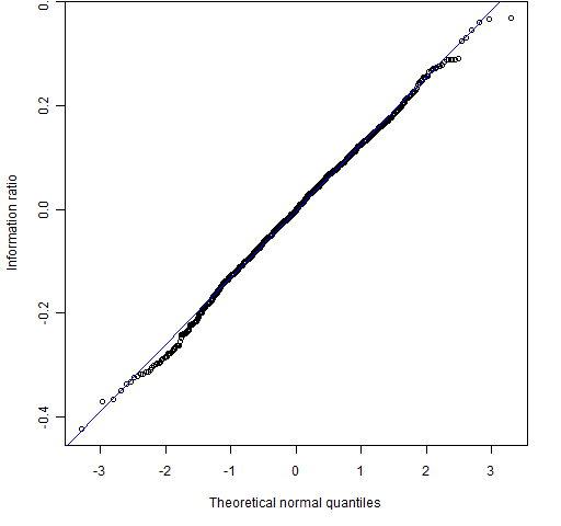
Figures 3 and 4 use the Cauchy distribution. This is more extreme than even the infinite variance gang believe. The Cauchy not only has an infinite variance, it has an infinite mean as well.
Figure 3: QQplot using 12 Cauchy distributed returns.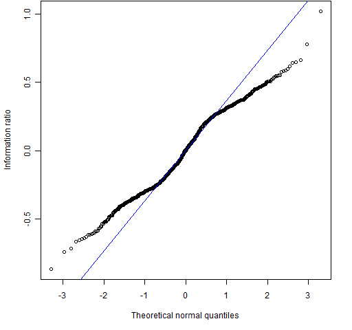
Figure 4: QQplot using 60 Cauchy distributed returns.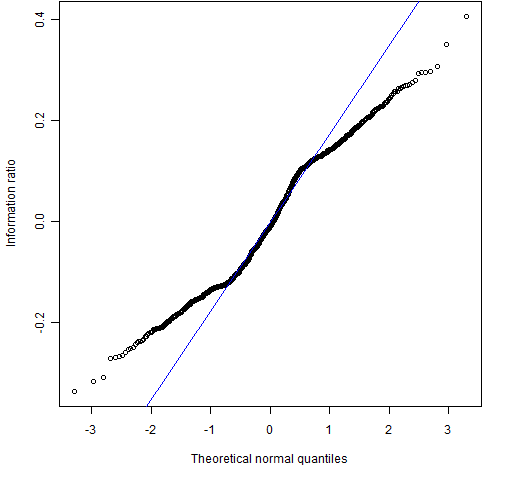
Figures 5 and 6 use Student’s t distribution with 1.5 degrees of freedom. This is more like the assumption that the infinite variance gang makes: infinite variance, finite mean.
Figure 5: QQplot using 12 t distributed (1.5 degrees of freedom) returns.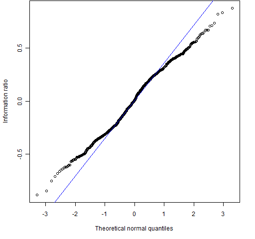
Figure 6: QQplot using 60 t distributed (1.5 degrees of freedom) returns.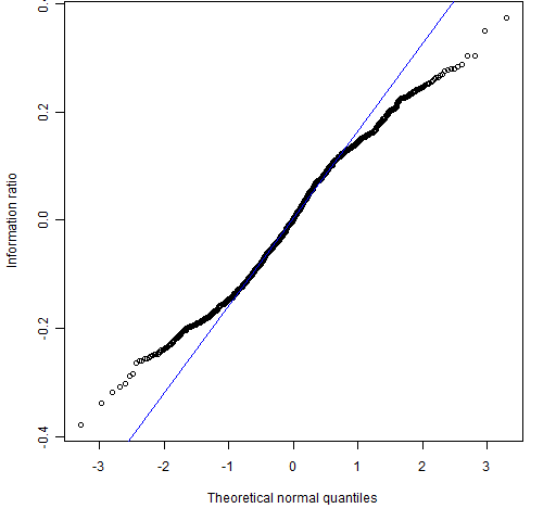
Figures 7 and 8 use Student’s t with 5 degrees of freedom. This, in my opinion, is a reasonable assumption for the distribution of daily returns.
Figure 7: QQplot using 12 t distributed (5 degrees of freedom) returns.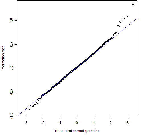
Figure 8: QQplot using 60 t distributed (5 degrees of freedom) returns.
Comments
The infinite variance distributions result in short-tailed distributions for the information ratio. Hence there should be no worry at all about the efficacy of the bootstrap in this situation.
These simulations implicitly assume that the information ratio is created with log returns rather than simple returns. There’s not likely to be much difference whichever returns are used.
The “reasonable” return distribution results in a distribution for the information ratio that is very close to normal. So you might ask what the advantage is of the bootstrap over traditional methods. One answer is that the bootstrap is probably better than analytic methods at handling whatever distortions there are from normality. Also with the bootstrap you don’t have to think — you only need to be able to write a for loop in R. That is, you can apply Uwe’s Maxim.
Epilogue
Who knows not where a wasp does wear his sting?
from The Taming of the Shrew by William Shakespeare
Appendix R
The data plotted in the figures were generated like:
ratio <- numeric(1000)
for(i in 1:1000) {
data <- rt(12, df=1.5)
ratio[i] <- mean(data) / sd(data)
}
It was then plotted (essentially) with:
qqnorm(ratio)
qqline(ratio, col="blue")
Those who believe that returns have infinite variance think they follow a stable distribution. There are functions for stable distributions in the fBasics and stabledist R packages.
I must take issue with applying Uwe’s Maxim in this case. While the determination of the proper distribution to use is thought intensive, I question whether that work is productive. By not making assumptions on distributions, we can focus on the variables that are far more important to decision makers such as rebalancing strategies and qualitative aspects of risk management. For long term investors, this may mean including “unreasonable” return distributions in order to increase certainty over factors that carry greater career risk.
Stephen, I’m confused by your first sentence. You are advocating bootstrapping so that you can save the hurt to think about more important things. Yes?
I am saying that we should attempt to get as close to perfection as possible because other aspects of the problem may not be perfect. Using the bootstrap ensures that there is 1 less problem that can occur in the analysis.