How well do asset weight constraints constrain risk?
The setup
In “Unproxying weight constraints” I claimed that many constraints on asset weights are really a proxy for constraining risk. That is not a problem if weights are a good proxy for risk. So the question is: how good of a proxy are they?
To give an answer to that we created a universe that is a non-random selection of about 400 stocks in the S&P 500. Using this data we generate random portfolios that use one or the other type of constraint. Then we can see the distributions of weights and risk fractions.
In all cases the random portfolios obey the constraints:
- long-only
- 40 to 50 names in the portfolio
In addition there is either the constraint:
- all asset weights less than 5%
or
- all asset risk fractions less than 5%
1000 random portfolios were generated in each case.
The variance matrix that is used is a Ledoit-Wolf shrinkage estimate (shrinking to equal correlation from the sample variance) based on about one year of daily data.
Results at 2008 Q3
The fourth quarter of 2008 was an exciting time in equities. We used data as of the end of the third quarter 2008.
Figure 1 exhibits the weights and the corresponding risk fractions of the assets in the portfolio that happened to be the first one generated with weight constraints.
Figure 1: Asset weights and risk fractions of the assets in a weight-constrained portfolio.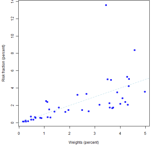
Figure 2 shows the distribution of risk fractions under the two constraint regimes.
Figure 2: 2008 Q3 distribution of all risk fractions when weight is constrained (blue line) and risk fraction is constrained (gold line).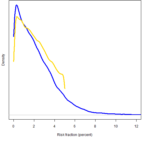 We see that there is an appreciable chance of the typical risk fraction being greater than 6%.
We get a different picture if we look at the maximum risk fraction in each portfolio rather than all of the risk fractions. Figure 3 shows that most portfolios have a fairly high maximum risk fraction — 5 out of the 1000 portfolios had a risk fraction over 20%.
Figure 3: 2008 Q3 distribution of maximum risk fraction when weights are constrained.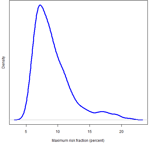 We can do the same sort of analysis on weights as on risk fractions. Figure 4 shows the distributions of all weights, and Figure 5 shows the distribution of maximum weights.
Figure 4: 2008 Q3 distribution of all weights when weight is constrained (blue line) and risk fraction is constrained (gold line).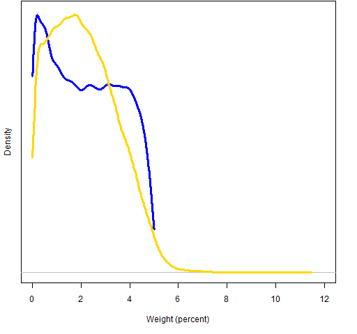
Figure 5: 2008 Q3 distribution of maximum weight when risk fractions are constrained.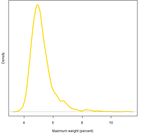
At least in this example, risk fraction is a good proxy for weight, but weight is not a good proxy risk.
Results at 2011 Q1
We’re currently experiencing more normal markets than in 2008. The same analysis was done as of 2011 March 31.
Figure 6: 2011 Q1 distribution of all risk fractions when weight is constrained (blue line) and risk fraction is constrained (gold line).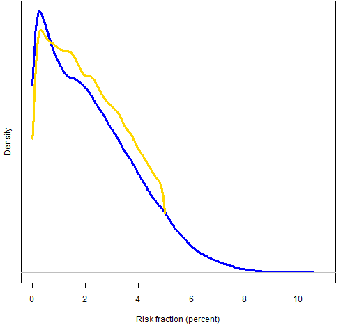
Figure 7: 2011 Q1 distribution of maximum risk fraction when weights are constrained.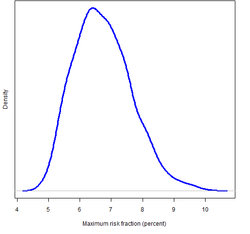
Figure 8: 2011 Q1 distribution of all weights when weight is constrained (blue line) and risk fraction is constrained (gold line).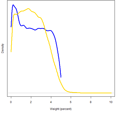
Figure 9: 2011 Q1 distribution of maximum weight when risk fractions are constrained.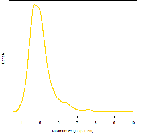
Appendix R
The full analysis (except for some of the plots) is in weightproxy.Rscript. Some of it is reproduced and explained here.
It starts off by using the QuantTrader blog post Downloading S&P 500 data to R. In particular the post includes a link to a file that contains the stock symbols for the constituents.
sp500.symbol.url <- "http://blog.quanttrader.org/wp-content/uploads/sp500.csv"
sp500.symbols <- scan(url(sp500.symbol.url), what="")
Then we source a file of functions related to the Portfolio Probe User’s Manual that includes a function to read multiple symbols. That function depends on the TTR package, which depends on the xts package.
source('https://www.portfolioprobe.com/R/pprobe_functions01.R')
require(TTR)
sp500.close <- pp.TTR.multsymbol(sp500.symbols, 20070101, 20110415)
sp500.close is a multivariate xts object. The pp.TTR.multsymbol function is simple-minded and throws away data that does not exactly fit the first data read. We continue to be simple-minded and just throw away those stocks.
sp500.closeok <- sp500.close[, colSums(is.na(sp500.close)) == 0]
I ended up with 392 stocks out of the 499 in the original list.
We create log returns from the closing prices:
sp500.ret <- diff(log(sp500.closeok))
Next we want to know where in the data the end of our selected quarter is. Here’s one way of doing it:
match("2008-09-30", as.character(index(sp500.ret)))
The as.character is an important piece of this command — it isn’t there just for looks.
Now we want to estimate a variance matrix using some data up to the end of the quarter. We do this with a function from the BurStFin package. If you don’t have BurStFin installed on your machine, then you can get it with the R command:
install.packages("BurStFin", repos="http://www.burns-stat.com/R")
Once the package is installed, do:
require(BurStFin)
sp500.var08Q3 <- var.shrink.eqcor(sp500.ret[seq(to=440, length=250),])
We will also need a price vector of the assets at the point in time that we are interested:
sp500.price08Q3 <- drop(as.matrix(sp500.closeok[440,]))
Now we are ready to generate the random portfolios. There is one more constraint not mentioned before, but it is really immaterial — the gross value of the portfolios are constrained to be (close to) 1 million dollars.
require(PortfolioProbe)
rp.08Q3.w05 <- random.portfolio(1000, prices=sp500.price08Q3, gross=1e6, long.only=TRUE, max.weight=.05, port.size=c(40,50))
rp.08Q3.rf05 <- random.portfolio(1000, prices=sp500.price08Q3, gross=1e6, long.only=TRUE, risk.fraction=.05, port.size=c(40,50), variance=sp500.var08Q3)
Now given the random portfolios we can get the weights and risk fractions:
rp.08Q3.w05.weights <- randport.eval(rp.08Q3.w05, FUN=function(x) valuation(x)$weight)
rp.08Q3.rf05.weights <- randport.eval(rp.08Q3.rf05, FUN=function(x) valuation(x)$weight)
rp.08Q3.rf05.rfrac <- randport.eval(rp.08Q3.rf05, keep="risk.fraction")
rp.08Q3.w05.rfrac <- randport.eval(rp.08Q3.w05, additional.args=list(risk.fraction=.05, variance=sp500.var08Q3), keep="risk.fraction")
