Some ways to explore how good a method of predicting returns is.

Data and model

The universe is 443 large cap US stocks that have data back to the beginning of 2004.  The daily (adjusted) close was used.

The model that is used as an example is the default signal from the MACD function of the TTR package in R.  As we’ll see, this works sometimes, and sometimes not.  The signal would need to be scaled to really be expected returns, but the scaling won’t matter for our tests.

Correlation with future returns

An easy thing to do is to look at the correlation across assets of the expected returns with future returns.  Figure 1 shows the correlation with the subsequent 20-day returns for times throughout the study period.

Figure 1: Correlation of MACD signal with 20-day subsequent returns at 20-day intervals. 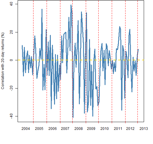The average correlation is close to zero, and there doesn’t seem to be much time dependence.  I suspect that the picture would improve for returns over longer periods.  That is merely unfounded speculation, and all the remaining examples will continue to use 20-day returns.

Figure 2 shows the scatterplot across stocks for the last available day.

Figure 2: MACD signal on 2013-01-16 versus the subsequent 20-day return with a lowess smooth. 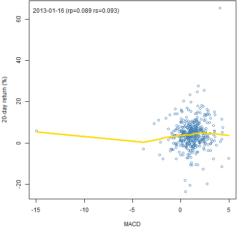The value marked “rp” is the Pearson (usual) correlation and the value marked “rs” is the Spearman (rank) correlation.  This plot makes it apparent that outliers can affect the smooth.  That’s not all bad — it is going to be the extreme cases that are most likely to show up in portfolios.

Figures 3 and 4 show some possible behaviors.

Figure 3: MACD signal on 2005-08-23 versus the subsequent 20-day return with a lowess smooth. 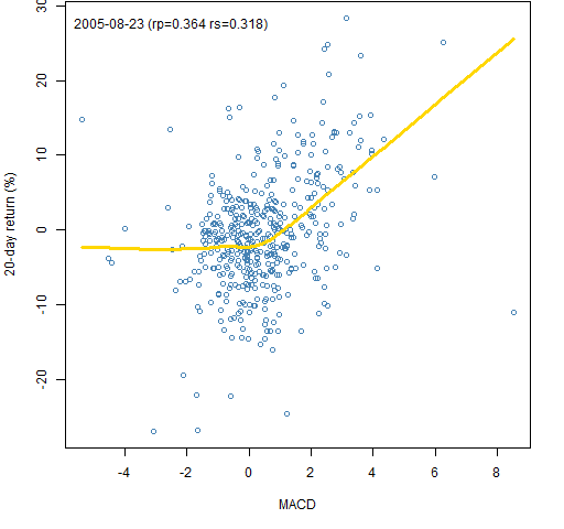This is an example where there is a response only on the positive side — no problem for a long-only portfolio.

Figure 4: MACD signal on 2005-12-15 versus the subsequent 20-day return with a lowess smooth. 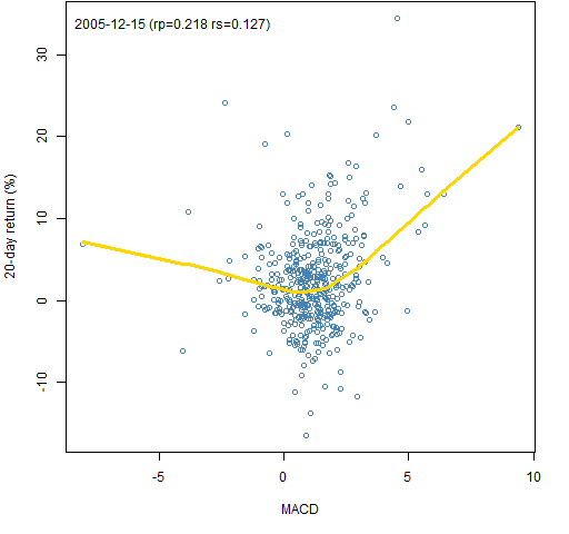Here we see that the response need not be monotone, and that the two correlation estimates need not be particularly close.

Looking at the tails

The assets that have the largest and smallest predicted returns are most likely to be selected to be in a portfolio.  We can compare the subsequent returns for the assets in the two tails by using boxplots.

Figures 5 through 7 do this for the same times as in Figures 2 through 4.

Figure 5: 20-day returns of the stocks with the 50 smallest and 50 largest MACD on 2013-01-16.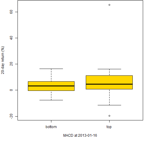

Figure 6: 20-day returns of the stocks with the 50 smallest and 50 largest MACD on 2005-08-23.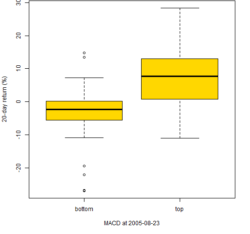

Figure 7: 20-day returns of the stocks with the 50 smallest and 50 largest MACD on 2005-12-15. 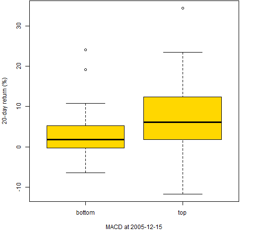In all three of these the top stocks have larger subsequent returns than the bottom stocks.  But we have selected times when the signal works.

Buy, sell, hold

So far we have assumed that we have a numerical prediction for the returns of each asset.  That is not always the case, especially with non-quant strategies.  Often assets are categorized as buy, sell or hold.  Or: strong buy, buy, hold, sell, strong sell.

Boxplots can be used in this situation as well.  Figures 8 through 10 use the same dates again and we artificially categorize the MACD.  The most extreme 50 are classified as strong buy or strong sell, the next 75 towards the center as buy or sell, and the remaining are classified as hold.

Figure 8: 20-day returns by classification on 2013-01-16.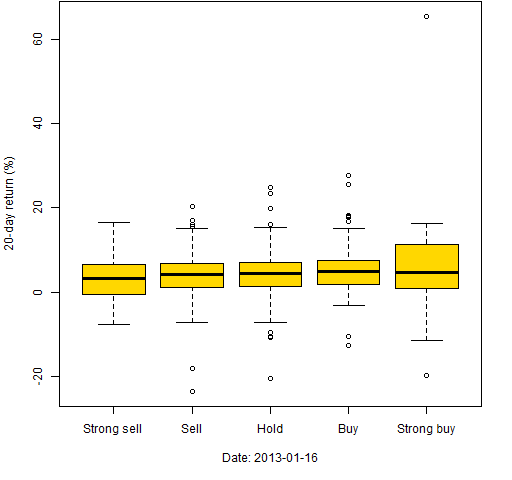

Figure 9: 20-day returns by classification on 2005-08-23.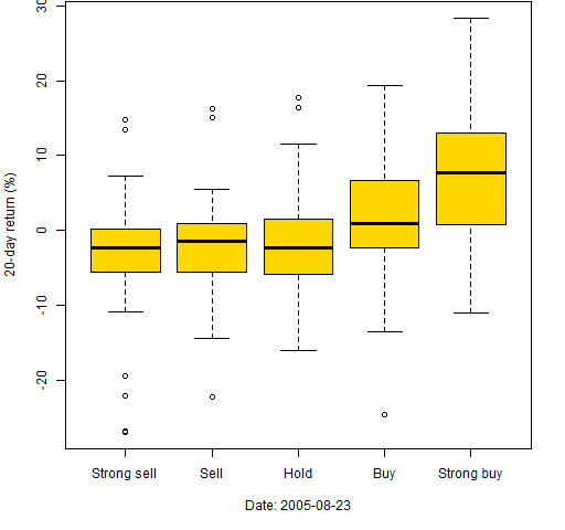

Figure 10: 20-day returns by classification on 2005-12-15.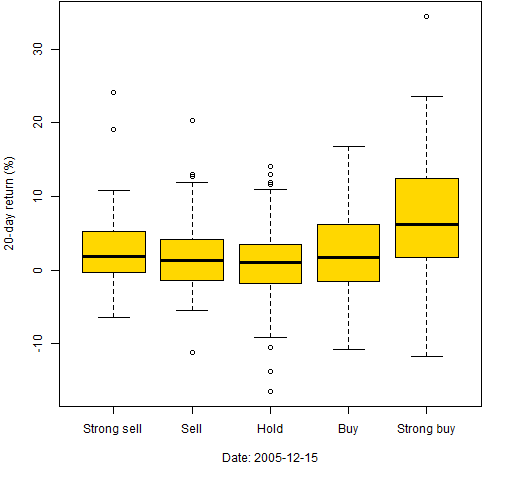

Other categories

All of these analyses can be done for subsets of the universe.  For instance, by sectors or by countries.

Related posts

• Again with variability of long-short decile tests
• Alpha decay in portfolios

Summary

There are easy ways to explore the quality of predicted returns for assets.

Appendix R

Computations were done in R.

match signal to returns

If we have a matrix of the predicted returns (assets in columns, times in rows) and a matrix of returns (with the same times and assets in the same order), then it is quite trivial in R to get matching subsequent returns for some length of time.  A simple loop will do.

macdcor <- rep(NA, nrow(univret130216))
names(macdcor) <- rownames(as.matrix(univret130216))

The commands above create a template for the object that will hold the time series of correlations between predicted returns and subsequent returns.  This is then used:

macdcor20 <- macdcor
tseq <- 1:20
for(i in 1:(length(macdcor20)-21)) {
  macdcor20[i] <- cor(univmacd130216[i,], 
                   colSums(univret130216[i+tseq,]))
}

This is using log returns.

If this were a more computationally intense procedure, we would probably want to only compute the correlation every twentieth day since that is all we ever use anyway.

The universe that is used here was selected so that there is data for all assets at all times.  That’s done to make the computations easier.  But when you are really doing this, you definitely don’t want to throw out assets just because they didn’t exist for the whole time period.  For this computation you would only need to specify an additional argument in the call to the correlation function to say to ignore missing values.

One of the best things about R is its handling of missing values.

getting the data in the first place

The initial collection of closing prices was created with:

initclose <- pp.TTR.multsymbol(univ00, 20040101, 20130104)

The market portraits from this year include a link showing how to get a collection of tickers for the S&P 500.

The function is defined as:

pp.TTR.multsymbol <- 
function(symbols, start, end, item="Close", adjust=TRUE,
    verbose=TRUE)
{
  fun.copyright <- "Placed in the public domain 2010-2012 by Burns Statistics"

  if(!length(symbols) || !is.character(symbols)) {
    stop("'symbols' needs to be a non-empty vector of characters")
  }
  require(TTR)
  init <- getYahooData(symbols[1], start=start, 
     end=end, quiet=TRUE, adjust=adjust)
  if(length(symbols) == 1) {
    ans <- xts(coredata(init)[, item], 
       order.by=index(init))
    attr(ans, "call") <- match.call()
    return(ans)
  }
  nobs <- nrow(coredata(init))
  if(nobs == 0) stop(paste("first symbol(", 
     symbols[1], ") failed", sep=""))
  ans <- array(NA, c(nobs, length(symbols)), 
     list(NULL, symbols))
  ans[,1] <- coredata(init)[, "Close"]
  if(verbose) {
    cat("done with:", symbols[1], " ")
    count <- 2
  }
  fail <- rep(FALSE, length(symbols))
  names(fail) <- symbols
  for(i in symbols[-1]) {
    this.c <- coredata(getYahooData(i, start=start, 
       end=end, quiet=TRUE, adjust=adjust))[, item]
    if(length(this.c) == nobs) {
      ans[, i] <- this.c
    } else {
      fail[i] <- TRUE
      # a careful implementation would 
      # put data in right spot
    }
    if(verbose) {
      count <- count + 1
      if(count %% 10 == 0) cat("\n")
      cat(i, " ")
    }
  }
  if(verbose) cat("\n")
  if(any(fail)) {
    warning(paste(sum(fail), 
       "symbols did not have the right number",
       "of observations -- the errant symbols are:",
       paste(symbols[fail], collapse=", ")))
  }
  ans <- xts(ans, order.by=index(init))
  attr(ans, "call") <- match.call()
  ans
}

updating closing prices

The initial data was purposely not up-to-date so that it could use the updating function:

univclose130216 <- pp.updateclose(initclose)
univret130216 <- diff(log(univclose130216))

This is naive in one sense and not naive in another.  It uses the function above that just throws out all data for an asset if it doesn’t have data at all the time points.  On the other hand, it checks an overlap period for agreement and gets the data for the entire time period for those assets where there is disagreement.  Disagreements occur when the adjustment changes.

The result is an xts object that is sort of but not exactly like a matrix.  Above there is a coercion to matrix which is done because the rownames of the matrix present the dates in a nicer fashion.

pp.updateclose <- function (univclose, overlap=5, 
   backup=FALSE) 
{
  # Placed in the public domain 2013 by Burns Statistics

  # Testing status: seems to work

  require(BurStMisc)

  today <- gsub("-", "", Sys.Date())

  if(backup) {
    save(univclose, file=paste("univclose_", today, 
       ".rda", sep=""))
  }
  start <- if(inherits(univclose, "zoo")) {
      tail(index(univclose), overlap)[1]
    } else {
      tail(rownames(univclose), overlap)[1]
   }
  start <- substring(gsub("-", "", start), 1, 8)
  newclose <- pp.TTR.multsymbol(colnames(univclose), 
     as.numeric(start), as.numeric(today))
  cc <- intersect(colnames(univclose), 
     colnames(newclose))
  if(nrow(univclose) < overlap) {
     overlap <- nrow(univclose)
  }
  ocom <- tail(univclose[, cc], overlap)
  ncom <- head(newclose[, cc], overlap)
  if(any(abs(ocom - ncom) / ocom > 1e-6)) {
    dif <- apply(abs(ocom - ncom) / ocom, 2, max)
    outnam <- cc[dif > 1e-6]
    replace <- pp.TTR.multsymbol(outnam, 
       as.numeric(gsub("-", "", index(univclose)[1])), 
       as.numeric(today))
  } else {
    outnam <- NULL
  }
  if(length(cc) < ncol(univclose)) {
    stop("new has fewer assets")
  }
  ans <- rbind(univclose, tail(newclose, -overlap))
  if(length(outnam)) {
    ans[, outnam] <- replace
    warning("changes to: ", paste(outnam, 
       collapse=", "))
  }
  print(cbind(corner(ans, 'bl', n=c(7,4)), 
     corner(ans, 'br', n=c(7,4))))
  ans
}

MACD

The signal is created with:

univmacd130216 <- pp.TTR.multmacd(univclose130216)

Using the function:

pp.TTR.multmacd <-
function (x, ...) 
{
    # placed in the public domain by 
    # Burns Statistics 2010-2011

    require(TTR)
    ans <- x
    ans[] <- NA
    for(i in seq(length=ncol(x))) {
      ans[,i] <- MACD(x[,i], ...)[, "signal"]
    }
    attr(ans, "call") <- match.call()
    ans
}

time plots

The function used to create Figure 1 is pp.timeplot which you can put into your R session with:

source("https://www.portfolioprobe.com/R/blog/pp.timeplot.R")

signal plots

Figures 2 through 4 were created with:

pp.signalReturnPlot <- function(index, times=20, 
    unit.time="day", name.signal="signal",
    signal=univmacd130216, retmat=univret130216)
{
  # placed in the public domain 2013 by Burns Statistics

  # testing status: seems to work

  if(is.character(index)) {
     index <- which(index == rownames(signal))
  }
  x <- signal[index,]
  y <- colSums(retmat[index + 1:times,]) * 100
  plot(x, y, col="steelblue", xlab=name.signal, 
     ylab=paste0(times,"-", unit.time, " return (%)"))
  lines(lowess(x,y), col="gold", lwd=3)
  pusr <- par("usr")
  text(pusr[1] + .02 * (pusr[2] - pusr[1]),
     pusr[3] + .95 * (pusr[4] - pusr[3]), 
     paste0(rownames(signal)[index], " (rp=", 
     round(cor(x,y), 3), " rs=", round(cor(x, y, 
     method="spear"), 3), ")"), adj=0)
}

tail plots

Figures 5 through 7 were created with:

pp.signalTailPlot <- function(index, times=20, 
    tailsize=50, unit.time="day", name.signal="signal",
    signal=univmacd130216, retmat=univret130216)
{
  # placed in the public domain 2013 by Burns Statistics

  # testing status: seems to work

  if(is.character(index)) {
     index <- which(index == rownames(signal))
  }
  x <- sort(signal[index,])
  xbot <- head(x, tailsize)
  xtop <- tail(x, tailsize)
  ybot <- colSums(retmat[index + 1:times, 
     names(xbot)]) * 100
  ytop <- colSums(retmat[index + 1:times, 
     names(xtop)]) * 100
  boxplot(list(bottom=ybot, top=ytop), col="gold", 
     ylab=paste0(times,"-", unit.time, " return (%)"),
     xlab=paste(name.signal, "at", 
     rownames(signal)[index]))

}