More risk does not necessarily mean bigger Value at Risk.
Previously
“The incoherence of risk coherence” suggested that the failure of Value at Risk (VaR) to be coherent is of little practical importance.
Here we look at an attribute that is not a part of the definition of coherence yet is a desirable quality.
Thought experiment
We have a distribution of returns that has a standard deviation of 1, and we vary the degrees of freedom. If the degrees of freedom are infinite, then we have the normal distribution.
As the degrees of freedom decrease, the tail lengthens. I think there is consensus that — conditional on the same standard deviation — a longer tail means more risk. Hence we want VaR to be larger for smaller degrees of freedom. Figure 1 shows that we almost have that for probability 1%.
Figure 1: Value at Risk with varying degrees of freedom of the t distribution for probability 1%. 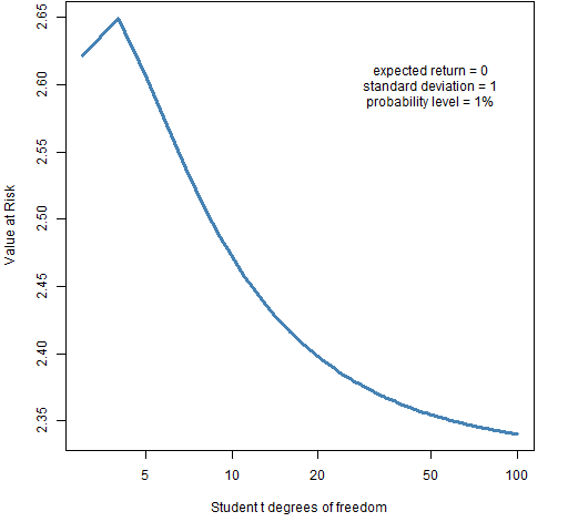 The VaR for 3 degrees of freedom is smaller than that for 4 degrees of freedom, but otherwise the plot is as we would hope — more risk means more VaR. Figure 2 adds Expected Shortfall to the picture.
Figure 2: Value at Risk and Expected Shortfall with varying degrees of freedom of the t distribution for probability 1%. 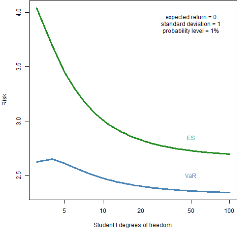 Expected Shortfall is well-behaved in this situation at least down to 3 degrees of freedom.
Now let’s change the probability level from 1% to 5%. Figure 3 shows the picture for VaR.
Figure 3: Value at Risk with varying degrees of freedom of the t distribution for probability 5%. 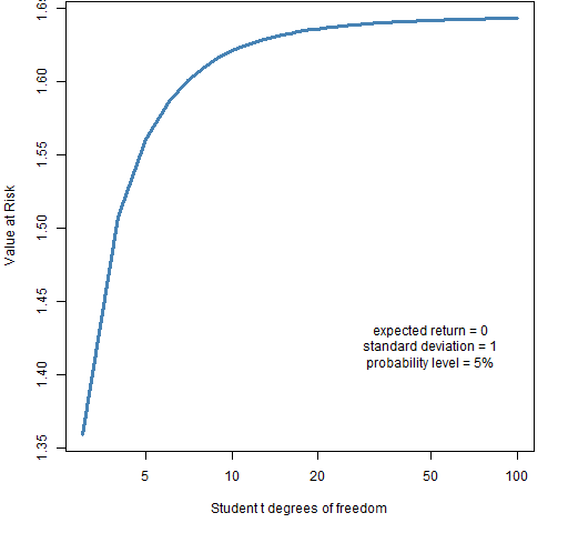 In Figure 3 we see precisely the wrong thing. The longer the tail, the smaller the VaR. Figure 4 shows Expected Shortfall as well for this case.
Figure 4: Value at Risk and Expected Shortfall with varying degrees of freedom of the t distribution for probability 5%. 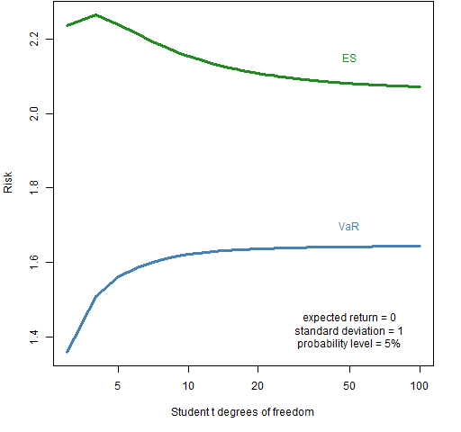 The Expected Shortfall breaks down going from 4 to 3 degrees of freedom, but otherwise has the proper orientation.
Figure 5 looks at the issue from a different point of view. Fix two distribution assumptions — in this case, t with 5 degrees of freedom and normal — and see how the difference changes as we vary the probability level.
Figure 5: t 5 degrees of freedom VaR minus normal VaR for varying probabilities. 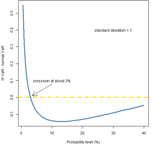 This shows that VaR doesn’t have the problem (with this pair of distributions) when the probability is less than 3%.
Summary
There is an irony that the normal distribution is a conservative assumption for Value at Risk with 5% probability.
Expected Shortfall is not entirely immune to this problem, but does much better than Value at Risk.
Epilogue
Oh Maybellene, why can’t you be true?
from “Maybellene” by Chuck Berry
Appendix R
The computing and graphics were done in the R language.
create Figure 2
The R function to produce Figure 2 is:
 function (filename = "risktdof01.png")
{
    if(length(filename)) {
        png(file=filename, width=512)
        par(mar=c(5,4, 0, 2) + .1)
    }
    dseq <- 3:100
    esseq <- sapply(dseq, es.tdistSingle, level=.01)
    matplot(dseq, cbind(-qt(.01, df=dseq) *
        sqrt((dseq - 2)/dseq), esseq), type="l",
        col=c("steelblue", "forestgreen"), lwd=3,
        log="x", lty=1, ylab="Risk",
        xlab="Student t degrees of freedom")
    text(50, 2.5, "VaR", col="steelblue")
    text(50, 2.85, "ES", col="forestgreen")
    text(50, 3.9,
        "expected return = 0\nstandard deviation = 1\nprobability level = 1%")

    if(length(filename)) {
        dev.off()
    }
}
The computations are done, the basic plot is done, and then pieces are added to the plot with additional commands.
compute Expected Shortfall
The function that computes the Expected Shortfall in the function above is:
es.tdistSingle <-
function (level, df, sd=1)
{
    # placed in the public domain 2013
    # by Burns Statistics

    # single ES value for t-distribution
    # testing status: slightly tested

    integ <- integrate(function(x) x * dt(x, df=df),
          -Inf, qt(level, df=df))$value
    -integ * sqrt((df-2)/df) * sd / level
}
sapply trick
There’s a command in the function that creates Figure 2 that is a little trickier than it might appear at first sight. The command is:
sapply(dseq, es.tdistSingle, level=.01)
Usually what is given to the function being applied in sapply (and lapply, apply and friends) is the first argument to the function. Subsequent arguments to the function may be passed in, like what is done in this case with level.
However, we’ve just seen that level is the first argument to the function. Since the first argument to the function is given, what is given to the function from dseq in the sapply command is the second argument. This is what we want — we want the values in dseq to represent degrees of freedom.
The command works because of the argument matching rules in R which are explained in Circle 8.1.20 of The R Inferno.
create Figure 5
The function for Figure 5 is:
function (filename = "VaRdiff.png")
{
  if(length(filename)) {
    png(file=filename, width=512)
    par(mar=c(5,4, 0, 2) + .1)
  }
  lseq <- seq(.005, .4, length=100)
  vdiff <- -qt(lseq, df=5)*sqrt(3/5) + qnorm(lseq)
  plot(lseq * 100, vdiff, type="l", col="steelblue",
       lwd=3, xlab="Probability level (%)",
       ylab="t5 VaR - normal VaR")
  abline(h=0, col="gold", lwd=3, lty=2)
  text(10, .1, "crossover at about 3%")
  arrows(10, .08, 3.5, .01)
  text(30, .4, "standard deviation = 1")

  if(length(filename)) {
    dev.off()
  }
}
Again, the computations are done, the basic plot is done, and then there are additions to the plot.

Hi Patric, very inspiring post!
I did some analysis to show why we are observing such behavior: A VaR paradox
Rocco,
Thanks for sharing that.
Pingback: Value at Risk with exponential smoothing | Portfolio Probe | Generate random portfolios. Fund management software by Burns Statistics