Specifics of statistical factor models and of a particular implementation of them.
Previously
Posts that are background for this one include:
- Three things factor models do
- Factor models of variance in finance
- The BurStFin R package
- The quality of variance matrix estimation
The problem
Someone asked me some questions about the statistical factor model in BurStFin. The response “I don’t know either” didn’t seem quite optimal.
The method
My way of getting to the answers was:
- Go back to the mathematical model
- Create a small, simple data example
Small data examples can be an effective way to clarify your thoughts. We’ll see that “small” means small for us, not necessarily small for the computer. That those can be different is part of the power of R.
The model
The post “Factor models of variance in finance” said:
In matrix notation a factor model is:
V = B’FB + D
This notation hides a lot of details:
- V is a square of numbers (of size number-of-assets by number-of-assets).
- B is a rectangle of sensitivities of size number-of-factors by number-of-assets.
- F is the variance matrix of the factors (of size number-of-factors by number-of-factors).
- D is a diagonal matrix (all off-diagonal elements are zero) of the idiosyncratic variance of each asset. The total size of D is number-of-assets by number-of-assets, but there are only number-of-assets values that are not zero.
(end quote)
But that is the model in terms of the variance matrix. The more fundamental model is in terms of the returns. We can write that as:
r = fB + e
where:
- r is a matrix of returns of size number-of-times by number-of-assets.
- f is a matrix of factor returns of size number-of-times by number-of-factors.
- B is a matrix of sensitivities of size number-of-factors by number-of-assets.
- e is a matrix of idiosyncratic (specific) returns of size number-of-times by number-of-assets.
The return equation looks suspiciously like a multivariate linear regression. In fact that is precisely how macroeconomic factor models are built. You could think of “f” as being the history of market returns, interest rates and so on; you would then do regressions to get the coefficients in B.
But we are doing a statistical factor model. The more proper name is a latent factor model. That is, we don’t get to see the factors — we only infer them. Since we are imagining the existence of phantoms, we might as well assume they are nice: we assume that they are uncorrelated with each other, and each has variance one. This means that “F” disappears from the first equation.
An example
Let’s use R to build a 2-factor model for 3 assets.
generate variance
The first thing to do is create a matrix of factor sensitivities:
set.seed(3)
realfac <- matrix(runif(6, -1,1), nrow=3)
The first command sets the seed for the random number generator so that the result will be reproducible. The second command creates a 3 by 2 matrix of random uniforms between -1 and 1.
It is traditional for there to be orthogonality between factors in statistical factor models. We can achieve that in our case by using the residuals from a linear regression:
realfac[,2] <- resid(lm(realfac[,2] ~ realfac[,1]))
The sensitivities are:
> realfac
           [,1]       [,2]
[1,] -0.6639169 -0.1563740
[2,]  0.6150328 -0.0802644
[3,] -0.2301153  0.2366384
Now we can create specific variances and the actual variance matrix:
realspec <- c(.04, .12, .32)
realvar <- realfac %*% t(realfac)
diag(realvar) <- diag(realvar) + realspec
The variance matrix is:
> realvar
           [,1]       [,2]       [,3]
[1,]  0.5052385 -0.3957794  0.1157734
[2,] -0.3957794  0.5047077 -0.1605221
[3,]  0.1157734 -0.1605221  0.4289508
generate returns
We’ll generate returns with a multivariate normal distribution with the variance that we’ve created. We’ll use a function from the MASS package to do that:
require(MASS)
retOneGo <- mvrnorm(1e6, mu=c(0,0,0), Sigma=realvar)
colnames(retOneGo) <- paste0("A", 1:3)
This creates a matrix that has 3 columns and 1 million rows. The last line names the assets.
The gore
We can now estimate a factor model from the returns:
require(BurStFin)
sfmOneGo <- factor.model.stat(retOneGo, weight=1,
           output="factor", range=c(2,2))
Often this function is called by just giving it the matrix of returns, but here we are overriding the default value of some arguments. By default the estimation uses time weights; saying “weight=1” is the easiest way of specifying equal weights. The default is to return the estimated variance matrix, here we are asking for the object containing the pieces to be returned. Finally we are demanding that exactly 2 factors be used.
The object is:
> sfmOneGo
$loadings
         [,1]       [,2]
A1  0.8617398 -0.3310512
A2 -0.8883301  0.2148856
A3  0.5923341  0.8038865
attr(,"scaled:scale")
[1] 0.728824 1.116636

$uniquenesses
        A1         A2         A3
0.14780966 0.16469372 0.03188738

$sdev
       A1        A2        A3
0.7119102 0.7111206 0.6551395

$timestamp
[1] "Sun Nov 11 10:07:19 2012"

$call
factor.model.stat(x = retOneGo, weights = 1,
    output = "factor", range.factors = c(2, 2))

attr(,"class")
[1] "statfacmodBurSt"
The components that pertain to the actual model are:
loadingsuniquenessessdev
sensitivities
The B in the equations above is:
> t(sfmOneGo$sdev * sfmOneGo$loadings)
             A1         A2        A3
[1,]  0.6134813 -0.6317098 0.3880615
[2,] -0.2356787  0.1528096 0.5266578
The operation to get this is to multiply each row of loadings by the corresponding element of sdev and then take the transpose.
specific variances
The uniquenesses are the fractions of the asset variances that are not explained by the factors. Thus the specific variances are the square of sdev times uniquenesses:
> sfmOneGo$sdev^2 * sfmOneGo$uniquenesses
        A1         A2         A3
0.07491232 0.08328438 0.01368631
orthogonality
Now let’s have a hunt for orthogonality. It is in the loadings:
> cov.wt(sfmOneGo$loadings, center=FALSE)
$cov
             [,1]         [,2]
[1,] 9.412928e-01 4.163336e-17
[2,] 4.163336e-17 4.010021e-01

$center
[1] 0

$n.obs
[1] 3
Note that the variance is the wrong thing to do here because it subtracts off the means:
> var(sfmOneGo$loadings)
            [,1]        [,2]
[1,]  0.88794845 -0.06484563
[2,] -0.06484563  0.32217545
The sensitivities including the standard deviations are not orthogonal:
> cov.wt(sfmOneGo$loadings * sfmOneGo$sdev, center=FALSE)
$cov
            [,1]        [,2]
[1,]  0.46300419 -0.01837012
[2,] -0.01837012  0.17813184

$center
[1] 0

$n.obs
[1] 3
This suggests that perhaps an option could be added to get orthogonality on this scale.
accuracy
We can see how close the estimate of the variance matrix is to the actual value. The estimated variance is:
> fitted(sfmOneGo)
           A1         A2         A3
A1  0.5068161 -0.4235562  0.1139464
A2 -0.4235562  0.5056925 -0.1646639
A3  0.1139464 -0.1646639  0.4416465
attr(,"number.of.factors")
[1] 2
attr(,"timestamp")
[1] "Sun Nov 11 10:07:19 2012"
The difference between the estimated variance and its true value is:
> fitted(sfmOneGo) - realvar
             A1            A2           A3
A1  0.001577602 -0.0277767353 -0.001826927
A2 -0.027776735  0.0009847477 -0.004141787
A3 -0.001826927 -0.0041417871  0.012695676
attr(,"number.of.factors")
[1] 2
attr(,"timestamp")
[1] "Sun Nov 11 10:07:19 2012"
The dfference between the estimate and the actual is small but not especially close to zero.
More gore (factor returns)
Now we’ll use the model we just estimated to simulate another set of returns. This time, though, we will create factor returns and idiosyncratic returns, and then put them together.
# generate factor returns ('f' in 2nd equation)
realFacRet <- matrix(rnorm(2e6), ncol=2)
# generate idiosyncratic returns ('e' in 2nd equation)
realFacSpec <- matrix(rnorm(3e6,
    sd=rep(sfmOneGo$sdev * sqrt(sfmOneGo$uniquenesses),
    each=1e6)), ncol=3)
# compute asset returns
retFR <- realFacRet %*% t(sfmOneGo$sdev *
    sfmOneGo$loadings) + realFacSpec
# name the assets
colnames(retFR) <- paste0("B", 1:3)
We use the new return matrix to estimate a factor model:
sfmFR <- factor.model.stat(retFR, weight=1,
     output="factor", range=c(2,2))
Now we can compare the sensitivities of the two models:
> t(sfmOneGo$sdev * sfmOneGo$loadings)
             A1         A2        A3
[1,]  0.6134813 -0.6317098 0.3880615
[2,] -0.2356787  0.1528096 0.5266578
attr(,"scaled:scale")
[1] 0.728824 1.116636
> t(sfmFR$sdev * sfmFR$loadings)
             B1         B2        B3
[1,]  0.6305413 -0.6505287 0.3757351
[2,] -0.2284438  0.1400226 0.5476813
attr(,"scaled:scale")
[1] 0.7171768 1.1040259
The "scaled:scale" attribute can be ignored.
We can estimate the factor returns implied by the newly estimated factor model. We have a multivariate regression but it is turned sideways from before. There are number-of-times individual regressions to do. Each of them have number-of-assets observations and number-of-factors coefficients to estimate. The coefficients will be our estimates of the factor returns.
As preparation, we create the matrix of sensitivities:
sensFRt <- sfmFR$sdev * sfmFR$loadings
Estimating a million regressions is more than we really want to do. Let’s do just the first 1000 observations in the return matrix:
 estFacRet <- t(coef(lm(t(retFR[1:1000,]) ~ 0 +
    sensFRt)))
This does a linear regression (lm) with the transpose of the first 1000 returns as the response and the sensitivities as the explanatory variables with no intercept. We then get the transpose of the coefficients of that regression.
We see that the variance matrix of the estimated factor returns is close to the identity — as we want:
> var(estFacRet)
            sensFRt1    sensFRt2
sensFRt1 1.015795719 0.007103762
sensFRt2 0.007103762 1.064414085
and that the variance of the errors of the factor return estimates is smaller:
> var(estFacRet - realFacRet[1:1000,])
            sensFRt1    sensFRt2
sensFRt1  0.07660990 -0.03752711
sensFRt2 -0.03752711  0.06754317
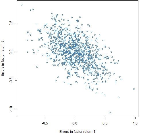
Plotting the errors shows that there can be fairly large discrepancies however.
Figure 1: The estimated factor returns minus the true factor returns for the first 1000 observations. 
It seems feasible to suppose that the regressions to get factor returns would be better in practice since there will be a large number of assets — the current case is estimating 2 parameters with only 3 observations. However, the estimation of the sensitivities will be worse since there will not be a million time points with which to estimate them (and the market is not going to follow the model anyway).
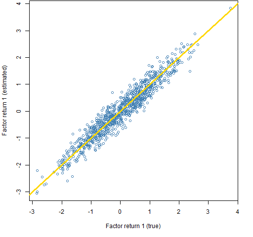
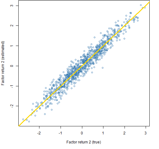
Figures 2 and 3 compare the true and estimated factor returns.
Figure 2: True and estimated returns for factor 1. 
Figure 3: True and estimated returns for factor 2. 
Questions
I’m thinking that statistical factor models have no advantages over a Ledoit-Wolf shrinkage estimate (var.shrink.eqcor in BurStFin). Hence enhancing factor.model.stat is a waste of time. Why am I wrong?
One of the features of the variance estimators in BurStFin is that they allow missing values. There is no guarantee that missing values are handled especially well. Would someone like to research how they should be handled? Please?

Hi Pat, great post! I went to talk in London not so long ago by a guy from MSCI/Barra who was touting their global model, which seemed to be factor models layered on factor models. They had geography and industry sector and instrument type etc. It occurred to me that while linear regression is numerically pretty well behaved, by the time you’ve composed a couple of layers of factor models your end result could be quite sensitive to changes in inputs. In which situation, surely a shrinkage approach would be better behaved?
Keiran,
Yes, shrinking towards something reasonable seems very likely to give a better model over all. But there’s a difference. Statistical factor models and Ledoit-Wolf are not able to give us information on sources of risk like industry and country. The two types of models have different uses.
There is an argument that the industry-etcetera models are better than statistical models because they bring in information in addition to the return history. That seems plausible to me, but I await evidence.
http://www.emis.de/journals/RCE/V34/v34n3a09.pdf
I’ve only skimmed this paper, but despite the text seeming to indicate the superiority of some form of statistical factor model over the shrinkage estimator, the actual results in the tables (particularly for when the number of assets is much larger than the number of time periods – “Table 2”) seem to show superior performance for the shrinkage estimator.
Jon,
Thanks for this. Yes, the text near Table 2 talks about shrinkage being better in the “very high dimensional” case of 500 assets. I see that as a mediocre dimensional case.