The paper is “Not Fooled by Randomness: Using Random Portfolios to Analyze Investment Funds” by Roberto Stein. Here is an explanation of the idea of random portfolios.
Favorite sentence
The real question here is whether we’re actually measuring skill, or these are still measures of performance, so influenced by extraneous factors that the existence of the funds manager’s skill cannot be ascertained.
Skill and performance are often conflated, but they are separate. Performance depends not only on skill but on the constraints that are faced.
Real data
The exciting part of the paper for me is the analysis of a group of U.S. equity mutual funds using monthly data from 2005 through 2010.
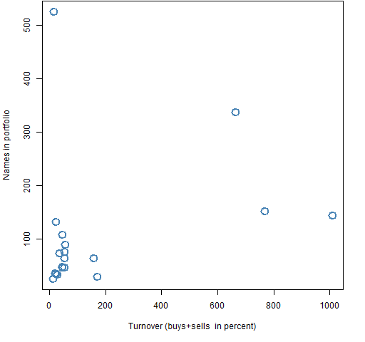
Figure 1 shows some information on the funds in the study.
Figure 1: Annual turnover and number of names in the funds that are studied. 
An executive summary is that there was reasonably good evidence that at least one (Jensen) of the 20 exhibited skill, but much less evidence of that once expenses are included. There were also two that showed negative skill over the time period, that is, seemed to actively destroy value for the investor.
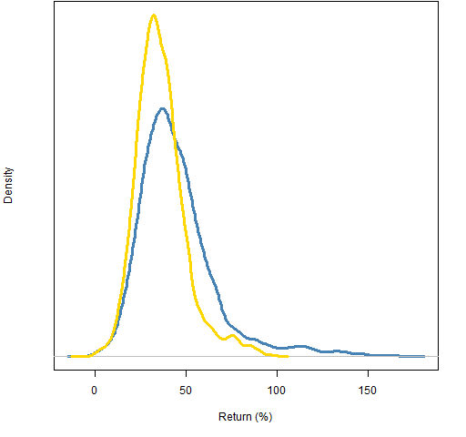
Figure 2 shows the returns for portfolios that have the constraints:
- assets from the constituents of the S&P 500
- no more than 100 names in the portfolio
- long-only
- maximum weight is 5% (at the start of 2006, there will be drift)
The returns are from the start of 2006 through 2011.
Figure 2: Distribution of random portfolio returns (2006-2011): simple returns (blue), log returns (gold).  The shape for the simple returns is very similar to Figure 1 in the Stein paper — they are both for 6 year periods, but they are a year off. This plot has 2011 instead of 2005.
We expect the simple returns to have a positive skew. Our prior for the log returns is that they might be symmetric.
Multi-fund models
The paper starts with a discussion of papers that use a bootstrap methodology on a universe of funds. In particular, the papers:
- Kosowski, R., Timmermann, A., Wermers, R., White, H., 2006, “Can Mutual Fund Stars Really Pick Stocks? New Evidence from a Bootstrap Analysis”, Journal of Finance, Vol. LXI, No. 6, 2551-2595. (SSRN version)
- Cuthbertson, K., Nitzsche, D., O’Sullivan, N., 2008, “UK mutual fund performance: skill or luck?”, Journal of Empirical Finance 15, 613-634. (SSRN version)
- Fama, E., K. French, 2010, “Luck versus skill in the cross-section of mutual fund returns”, Journal of Finance, Vol. LXV-5, 1915-1947. (SSRN version)
The techniques of these papers have several problems:
- They demand having data on a big universe of funds.
- They depend on a model of fund returns.
- They implicitly assume that all funds face similar constraints.
- Even if the above were not problems, you don’t get specific information about any particular fund.
In contrast, evaluating skill with random portfolios is much simpler and more informative.
Constrained random portfolio analysis
One methodology for assessing fund management skill with random portfolios is:
- Do random trades through the evaluation period starting with the positions held by the fund at the start of the period. The trades obey the fund constraints and mimic the turnover of the fund (and cash flow, if known).
- Repeat step 1 multiple times.
- Compare the period return of the fund to the distribution of returns of the random portfolios.
The portfolios created in the first two steps are pure luck given the decisions that the fund actually faced. We infer skill if the real fund does not look like it fits in the “luck” distribution. More color on this methodology can be found at this performance measurement page.
The Stein paper introduces an alternative way of using random portfolios to distinguish skill from luck. A limitation of the technique just described is that it only uses the return for the whole period. It throws away all the information about how that was achieved.
The paper describes a means of using the whole series of returns within the period. Steps 1 and 2 remain the same. Step 3 is more complicated.
Conclusion
The final sentence of the paper is one that I agree with:
In all, [random portfolio analysis] is an important addition to the finance analysis toolkit.
Appendix R
read in data from a table in pdf
The data to get Figure 1 was taken out of the paper by (in Windows) copying the body of Table I to the clipboard and then doing the R command:
notFoolFunds <- matrix(readClipboard(), nrow=20,
   byrow=TRUE)
This is a chararcter matrix but we are really interested in the numbers. So make a new matrix with the two columns we care about and modify the result to be numeric:
notFoolFundsNum <- notFoolFunds[, 4:5]
mode(notFoolFundsNum) <- "numeric"
Figure 1 is sort of:
plot(notFoolFundsNum)
random portfolio returns
The random portfolios for Figure 2 were generated (10,000 of them) by:
require(PortfolioProbe)
rp100w05 <- random.portfolio(1e4, prices=sp5.close[1,],
   gross=1e6, long.only=TRUE, port.size=100,
   max.weight=.05)
Then the returns are computed:
sret.rp100w05 <- valuation(rp100w05,
   prices=sp5.close[c(1,1511),], returns="simple")
lret.rp100w05 <- valuation(rp100w05,
   prices=sp5.close[c(1,1511),], returns="log")
Of course, we could have just transformed the simple returns into log returns or vice versa.
A plot of the density of the simple returns is:
plot(density(sret.rp100w05 * 100))
