How much predictability is there for these higher moments?

Data

The data consist of daily returns from the start of 2007 through mid 2011 for almost all of the S&P 500 constituents. Estimates were made over each half year of data.  Hence there are 8 pairs of estimates where one estimate immediately follows the other.

What is more important than predicting actual values — at least for such applications as portfolio optimization — is predicting the rank within the universe.  Hence looking at the Spearman correlation between estimates in different time periods is a reasonable test of the predictability that we care about.

Kurtosis

There’s good news and bad news.

Figure 1 shows the good news — there is statistically significant predictability in kurtosis.

The kurtosis estimates are in a matrix: 9 columns for different times and 477 rows for the assets.  The steps of the permutation test were:

• Do 1000 times:  permute the values within each column (so the values in any row  of the permuted data are for different assets)
• Save the 8 correlations in sorted order from each of the permuted matrices
• Save the sorted correlations from the original data

This is then plotted in Figure 1.  The boxplots show the distributions of the correlations from the permuted data (the boxplot at 1 is the distribution of the smallest correlations, the boxplot at 8 is the distribution of the largest correlations).  The blue points show the actual correlations.  The distribution of actual correlations is unambiguously larger than what would happen by chance.

Figure 1: Permutation test of Spearman correlation between contiguous pairs of kurtosis estimates, sorted — actual data are in blue.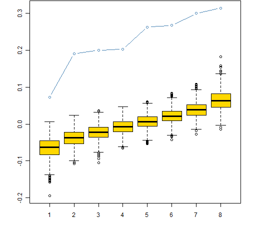 
The bad news is that it seems doubtful that the predictability is of economic significance.  Figure 2 shows the most recent pair of estimates.  This looks typical but happens to be the one with the largest Spearman correlation.  Figure 3 is the same data plotted on log scales.

Figure 2: Estimates of kurtosis for data starting mid 2010 and starting at the start of 2011.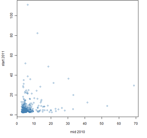

Figure 3: Estimates of kurtosis for data starting mid 2010 and starting at the start of 2011, log scales. 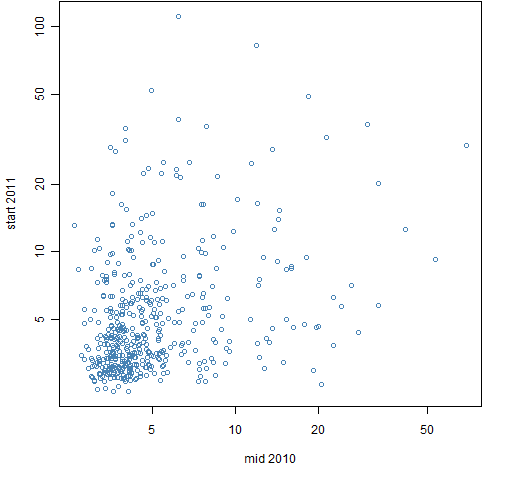To give a sense of perspective, Figure 4 shows the corresponding data for volatility.

Figure 4: Estimates of volatility for data starting mid 2010 and starting at the start of 2011.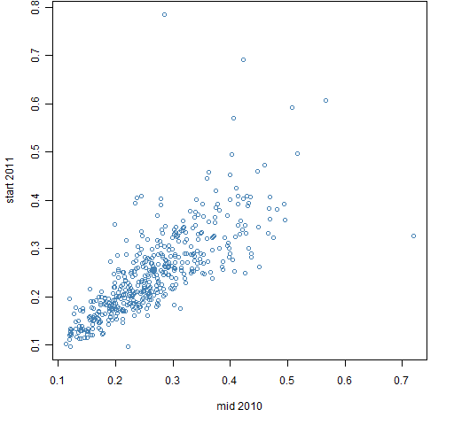

Skewness

Figure 5 shows the results of the permutation test on skewness estimates.  The observed correlations look just like a typical result from the permuted data.

Figure 5: Permutation test of Spearman correlation between contiguous pairs of skewness estimates, sorted — actual data are in blue.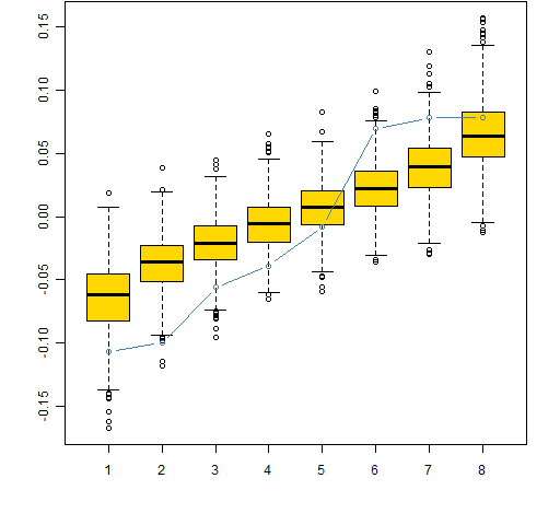
This does not prove that there is no predictability in skewness.  It does, however, suggest that — just as with expected returns — looking for predictability based only on the past price history is unlikely to be fruitful.

Questions

What other ways are there to explore kurtosis and skewness?

Using a year rather than half a year of data seems to make little difference.

Appendix R

estimation

The first task is to create the matrices that will hold the estimates:

spHkurt <- spHskew <- array(NA, c(477, 9), list(colnames(spmat.ret)[-1], names(sp.breakr)[-10]))

Then the matrices are populated:

for(i in 1:9) spHkurt[,i] <- pp.kurtosis(spmat.ret[seq(sp.breakr[i], sp.breakr[i+1]), -1])

for(i in 1:9) spHskew[,i] <- pp.skew(spmat.ret[seq(sp.breakr[i], sp.breakr[i+1]), -1])

The reason that the first column of the returns data is dropped is because that column holds the returns for the index.  (There is an off-by-one error in the seq commands above, but that is the code that was actually used.)

permutation test

The permutation tests are done with:

perm.spcorHkurt <- pp.corcolperm(spHkurt)
perm.spcorHskew <- pp.corcolperm(spHskew)

plot

Figure 1 was created by:

boxplot(perm.spcorHkurt$perms, col="gold",  ylim=range(perm.spcorHkurt$perms, perm.spcorHkurt$statistic))

points(1:length(perm.spcorHkurt$statistic), perm.spcorHkurt$statistic,  col='steelblue', type='b')

source code

The definitions of the skewness, kurtosis and permutation functions are in kurtskew.R

Update: the original version of this file had a bug in the function (the data were not properly centered).  It was updated 2012-04-29.  The numerical values in this post are off, but the patterns should be the same.

Subscribe to the Portfolio Probe blog by Email