Investment Performance Guy had a post about beta equal 1.  It made me wonder about the properties of portfolios with beta equal 1.  When I looked, I got a bigger answer than I expected.

Data

I have some S&P 500 data lying about from the post ‘On “Stock correlation has been rising”‘.  So laziness dictated that I use that.

It is daily data.  I used 2010 to estimate the betas.  The first half of 2011 is the out-of-sample period.

Figure 1: Distribution of S&P 500 betas estimated from 2010 daily data. 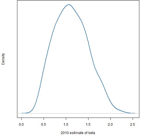Figure 2: 2011 H1 returns versus 2010 estimates of beta with the default lowess fit. 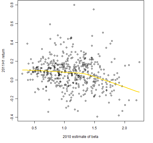Figure 2 shows a tendency for returns to decrease with beta.  Theory says they should be increasing.  This picture is one more circumstantial piece of evidence that low volatility investing is useful.  Falkenblog just posted “Beta Adored Before Data” that gives some historical perspective on Figure 2.

Two sets of random portfolios were created.  There were 10,000 long-only portfolios in each set and in each case the portfolio beta was restricted to be between 0.99 and 1.01.  One set  consisted of portfolios with 20 assets, the other set had 200 assets per portfolio.

Returns

Figures 3 and 4 show the distribution of returns for the first half of 2011 of the two sets of random portfolios.  The return of the index for the period is ever so close to 5%.

Figure 3: Distribution of 2011 H1 returns for portfolios with 20 assets and beta from 0.99 to 1.01.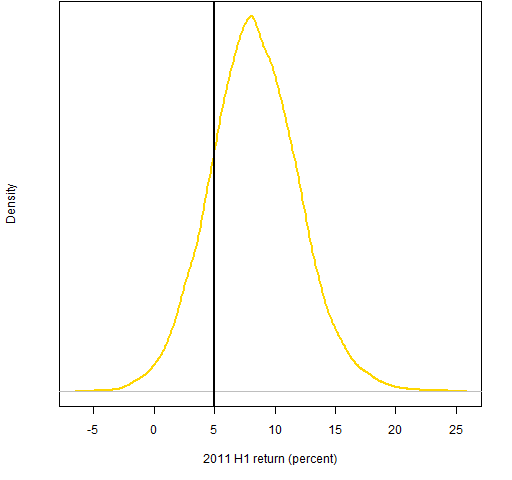

Figure 4: Distribution of 2011 H1 returns for portfolios with 200 assets and beta from 0.99 to 1.01.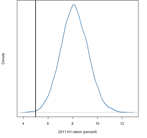

Surprising.

Corroboration

The first thing to do when you get a surprising result is to wonder what you’ve done wrong.

I looked.  Didn’t see anything.

I then created some random portfolios “by hand” that satisfy beta equal 1.  This had two steps:

1. Select the correct number of assets at random.
2. Equal weight the assets with betas less than 1 and equal weight the assets with betas greater than 1 such that the beta is 1.

The distributions of returns for the 20 asset portfolios are very similar (even though they have different restrictions on weights).  The equal weighted distribution for 200 assets has the same center but is narrower — meaning the index return looks even more out of place.

Volatility and information ratio

The realized volatility for the S&P 500 for the first half of 2011 is about 12.9%.  Figures 5 and 6 show the volatility distributions of the random portfolios.

Figure 5: Distribution of 2011 H1 realized volatility for portfolios with 20 assets and beta from 0.99 to 1.01.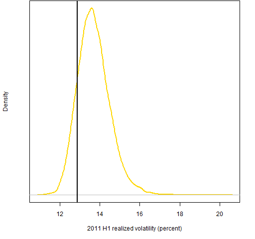

Figure 6: Distribution of 2011 H1 realized volatility for portfolios with 200 assets and beta from 0.99 to 1.01. 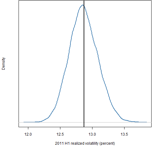Figures 7 and 8 show the information ratios for the random portfolios.  The index got a 5% return in half a year with about 13% (annualized) volatility, so the information ratio of the index was roughly 0.8.

Figure 7: Distribution of 2011 H1 information ratio for portfolios with 20 assets and beta from 0.99 to 1.01.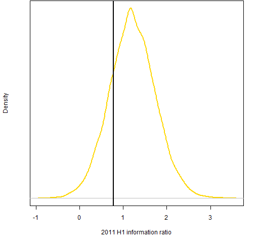

Figure 8: Distribution of 2011 H1 information ratio for portfolios with 200 assets and beta from 0.99 to 1.01.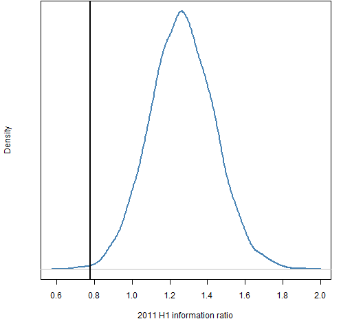 

These graphs are suggestive that the index is not on the efficient frontier.

Summary

Constraining beta to be close to 1 does not make portfolios behave like the index.  This seems to be another myth to add to the 4.5 myths about beta in finance.

Appendix R

estimate beta

It is shockingly easy in R to get the betas for a cohort of assets.  Once you have a matrix of the asset returns (times in the rows, assets in columns) and a vector of the market returns at the same times, it is one line:

spbeta <- coef(lm(spcon2010 ~ spx2010))[2,]

The creation of the original data can be seen at ‘On “Stock correlation has been rising”‘. Subsets of the original data were then created to fit our purpose here.

prepare to generate random portfolios

require(PortfolioProbe)

spbetacon <- build.constraints(spbeta)
spbetabounds <- spbetacon$bounds
spbetabounds[] <- c(.99, 1.01)
sp.price2011 <- as.matrix(sp500.close)[1007, names(spbeta)]

actually generate random portfolios

ran.spb1.200 <- random.portfolio(1e4, sp.price2011, gross=1e6, long.only=TRUE, lin.constraint=spbetacon$lin.constraints, lin.bound=spbetabounds, port.size=c(200,200))

use random portfolios

val.spb1.200 <- valuation(ran.spb1.200, spclose2011H1, collapse=TRUE)

The object created above is a matrix with the value of the portfolios (10,000 columns) for each day in the first half of 2011 (126 rows).

ret.spb1.200 <- pp.simpret(val.spb1.200[c(1,126),])
plot(density(ret.spb1.200)) # basis of Figure 4
plot(density(sqrt(252) * sd(diff(log(val.spb1.200)))))

Subscribe to the Portfolio Probe blog by Email