
The effect of beta equal 1
August 29, 2011
Investment Performance Guy had a post about beta equal 1. It made me wonder about the properties of portfolios with beta equal 1. When I looked, I got a bigger answer than I expected.
Data
I have some S&P 500 data lying about from the post ‘On “Stock correlation has been rising”‘. So laziness dictated that I use that.
It is daily data. I used 2010 to estimate the betas. The first half of 2011 is the out-of-sample period.
Figure 1: Distribution of S&P 500 betas estimated from 2010 daily data. 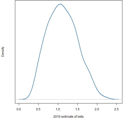 Figure 2: 2011 H1 returns versus 2010 estimates of beta with the default lowess fit.
 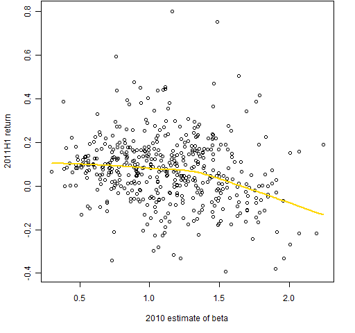 Figure 2 shows a tendency for returns to decrease with beta. Theory says they should be increasing. This picture is one more circumstantial piece of evidence that low volatility investing is useful. Falkenblog just posted “Beta Adored Before Data” that gives some historical perspective on Figure 2.
Two sets of random portfolios were created. There were 10,000 long-only portfolios in each set and in each case the portfolio beta was restricted to be between 0.99 and 1.01. One set consisted of portfolios with 20 assets, the other set had 200 assets per portfolio.
Returns
Figures 3 and 4 show the distribution of returns for the first half of 2011 of the two sets of random portfolios. The return of the index for the period is ever so close to 5%.
Figure 3: Distribution of 2011 H1 returns for portfolios with 20 assets and beta from 0.99 to 1.01. 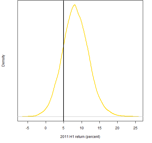
Figure 4: Distribution of 2011 H1 returns for portfolios with 200 assets and beta from 0.99 to 1.01. 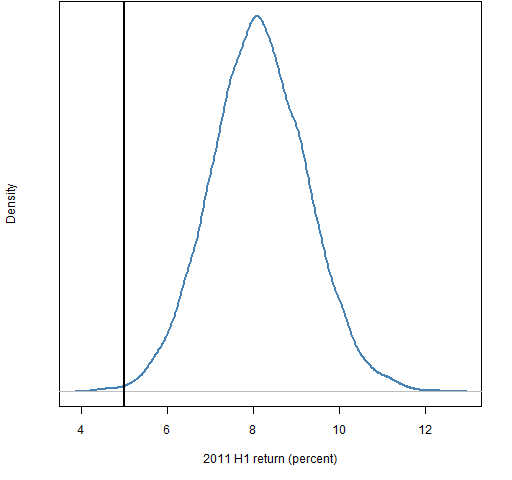
Surprising.
Corroboration
The first thing to do when you get a surprising result is to wonder what you’ve done wrong.
I looked. Didn’t see anything.
I then created some random portfolios “by hand” that satisfy beta equal 1. This had two steps:
- Select the correct number of assets at random.
- Equal weight the assets with betas less than 1 and equal weight the assets with betas greater than 1 such that the beta is 1.
The distributions of returns for the 20 asset portfolios are very similar (even though they have different restrictions on weights). The equal weighted distribution for 200 assets has the same center but is narrower — meaning the index return looks even more out of place.
Volatility and information ratio
The realized volatility for the S&P 500 for the first half of 2011 is about 12.9%. Figures 5 and 6 show the volatility distributions of the random portfolios.
Figure 5: Distribution of 2011 H1 realized volatility for portfolios with 20 assets and beta from 0.99 to 1.01. 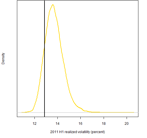
Figure 6: Distribution of 2011 H1 realized volatility for portfolios with 200 assets and beta from 0.99 to 1.01. 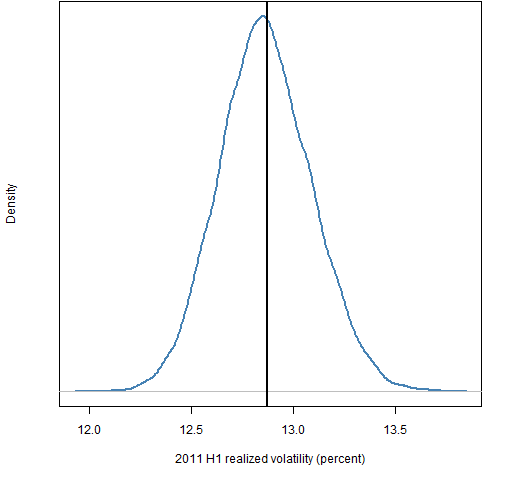 Figures 7 and 8 show the information ratios for the random portfolios. The index got a 5% return in half a year with about 13% (annualized) volatility, so the information ratio of the index was roughly 0.8.
Figure 7: Distribution of 2011 H1 information ratio for portfolios with 20 assets and beta from 0.99 to 1.01. 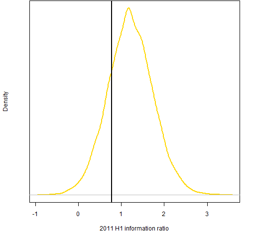
Figure 8: Distribution of 2011 H1 information ratio for portfolios with 200 assets and beta from 0.99 to 1.01. 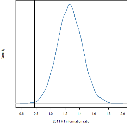
These graphs are suggestive that the index is not on the efficient frontier.
Summary
Constraining beta to be close to 1 does not make portfolios behave like the index. This seems to be another myth to add to the 4.5 myths about beta in finance.
Appendix R
estimate beta
It is shockingly easy in R to get the betas for a cohort of assets. Once you have a matrix of the asset returns (times in the rows, assets in columns) and a vector of the market returns at the same times, it is one line:
spbeta <- coef(lm(spcon2010 ~ spx2010))[2,]
The creation of the original data can be seen at ‘On “Stock correlation has been rising”‘. Subsets of the original data were then created to fit our purpose here.
prepare to generate random portfolios
require(PortfolioProbe)
spbetacon <- build.constraints(spbeta)
spbetabounds <- spbetacon$bounds
spbetabounds[] <- c(.99, 1.01)
sp.price2011 <- as.matrix(sp500.close)[1007, names(spbeta)]
actually generate random portfolios
ran.spb1.200 <- random.portfolio(1e4, sp.price2011, gross=1e6, long.only=TRUE, lin.constraint=spbetacon$lin.constraints, lin.bound=spbetabounds, port.size=c(200,200))
use random portfolios
val.spb1.200 <- valuation(ran.spb1.200, spclose2011H1, collapse=TRUE)
The object created above is a matrix with the value of the portfolios (10,000 columns) for each day in the first half of 2011 (126 rows).
ret.spb1.200 <- pp.simpret(val.spb1.200[c(1,126),])
plot(density(ret.spb1.200)) # basis of Figure 4
plot(density(sqrt(252) * sd(diff(log(val.spb1.200)))))

I’m an amateur when it comes to portfolio management, so I’ll tread lightly here.
But the most straight-forward explanation is that CAPM is not all that, well, true. The conjecture that “More Beta = More Returns” assumes that the market rationally trades off risk and reward.
However, “More Beta = Less Returns” makes perfect sense in light of how markets can chase speculative, non-fundamental and short sellers do not have enough liquidity or patience to correct the speculation. Growth stocks, in particular, have business models which make their fundamental valuation more ambiguous. The ambiguity, in turn, makes the stocks more susceptible to good stories which drive bubbles, such as “mind share” in the tech bubble. Meanwhile, low-beta value stocks have boring business models which have less ambiguity in their fundamental valuations. They have less susceptibility to speculative bubbles and thus have less susceptibility to investors overpaying.
Since CAPM has correlations based on past data which feed back on itself, it’s tough to really test this theory out. Growth stocks, for example, have big issues with survivorship bias (Google’s around and pets.com isn’t). But this theory and the data in this post make much more sense to me than basic CAPM, where valuations are always correct and ration. Yes, it’s extremely tough to make money in the market and actively-managed funds mostly do not make up for fees and transaction costs, but it does not follow that valuations always make sense. Bubbles can still happen because it’s very tough and dangerous to short-sell the market.
Matt,
Yes, that is perhaps the leading explanation for high beta (or volatility) assets to have lower expected returns.
Another explanation (both could be true) is that people who want to leverage buy the high volatility assets and hence push down their expected returns.
The preponderance of evidence for the low-volatility “anomaly” notwithstanding, another possible explanation for this particular exercise may be that historical beta is not the best forecast of future beta (versus forecasts based on a fundamental factor model), especially if the portfolio is only rebalanced once per year.
That said, anyone who really desired index-like performance would constrain more than just beta, but your point is certainly well-taken. Fundamental managers who’ve begun to implement quantitative risk management techniques (of which there seem to be an increasing number) would be well-advised not to do so naively.
Michael,
Thanks for your comments. How best to predict beta is an interesting question. But given that I don’t think beta should play a very important role, I’d relegate it to being an academic question. Certainly for the portfolios of size 200 the current beta prediction is doing okay at the portfolio level.
I agree that hopefully more constraints than just beta are imposed to try to imitate indices, though I’m not a big fan of imitating indices.
As mentioned in earlier comments, you could just be seeing the results of poor beta estimation. There are entire products out there that are intended to help forecast beta and these products are quite expensive, which indicates to me that the problem of forecasting beta is quite real and quite difficult.
Perhaps these results would be much more sound if you were to re-run this experiment with the benefit of perfect foresight. In other words, instead of estimating beta by using a linear regression on historical returns, why not set your beta forecast equal to the actual realized beta in out-of-sample? I know, using info from the future is typically frowned upon, but you are not backtesting an alpha strategy here, so you should be OK.
If you were able to reproduce your results, even after using perfect betas, then that would be a much stronger statement. In fact, it would easily dismiss some of the questions from comments above that essentially boil down to — “well your results seem reasonable, but you don’t use the great beta estimates from Vendor X that I do so you must be wrong.”
Thanks for the comment. I’ve put your suggestion of using look-ahead betas on my list of possible blog topics. So maybe some day …