
Variability in maximum drawdown
June 4, 2012
Maximum drawdown is blazingly variable.
Psychology
Probably the most salient feature that an investor notices is the amount lost since the peak: that is, the maximum drawdown.
Just because drawdown is noticeable doesn’t mean it is best to notice.
Statistics
The paper “About the statistics of the maximum drawdown in financial time series” explores drawdown analytically. The interesting part for me is Figures 14 onwards (which start on page 14). The pictures imply that the maximum drawdown could have been pretty much anything.
In the post “A minimum variance portfolio in 2011” we explored a particular portfolio. Figure 1 shows its value through 2011. We’ll use this as our example.
Figure 1: The value of the portfolio throughout 2011. 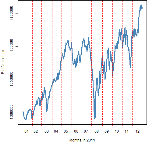
The maximum drawdown of this portfolio is 11.1%.
It is almost true that we shouldn’t care what order the returns arrive in as long as we get the same set of returns over the year. In other words, we should be just as happy with each permutation of the order of the returns of our portfolio.
Figure 2 shows the maximum drawdown distribution for random permutations of the returns of our portfolio. Remember that the return over the year is precisely the same for all the portfolios with these drawdowns.
Figure 2: Distribution of maximum drawdown from permutations of the portfolio returns, with 95% confidence interval (gold lines). 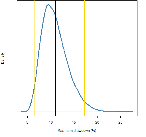 We can easily get maximum drawdowns from 7% to 17% using the exact same returns.
Given the big drop at the beginning of August, we might be led to think that the real maximum drawdown would be large relative to the possibilities over the permutations. Actually it is only slightly larger than the mean.
What do worst-case and best-case profiles look like? Figure 3 shows a permutation that comes close to maximizing the drawdown and Figure 4 shows one that comes close to minimizing drawdown.
Figure 3: Permutation of the portfolio returns that produces a large drawdown. 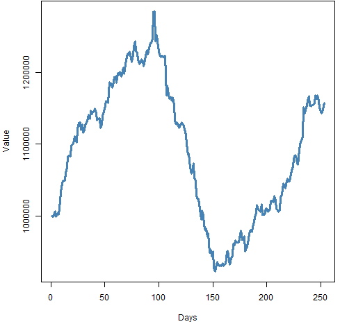
Figure 4: Permutation of the portfolio returns that produces a small drawdown. 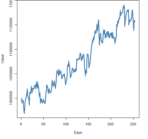
Large drawdowns occur when the negative returns are all bunched together. Small drawdowns happen when the negative returns are evenly spread.
Above I said we should be almost indifferent to different permutations of the returns. The catch is that we need to believe that there is neither momentum nor mean-reversion. In Figure 3 we have selected for momentum, and we have selected for mean-reversion in Figure 4.
You may be wondering what the equivalent pictures to Figures 3 and 4 are when the overall return is negative. Obviously the maximum drawdown has to be at least as big as the overall loss. To get big drawdowns the strategy remains the same — push all the negative returns together.
Figure 5 shows an example of minimizing the maximum drawdown when there is an overall loss — create multiple drawdowns of the same size. That is the strategy with overall gains as well, but less obvious on first sight.
Figure 5: Permutation of the negative portfolio returns that produces a small drawdown. 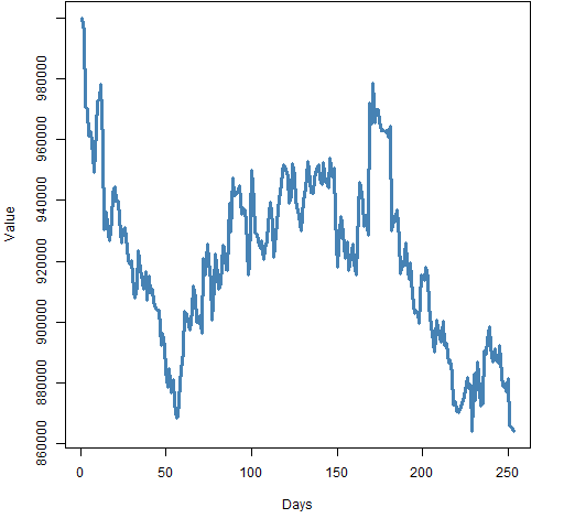
Summary
While maximum drawdown is emotionally compelling, it is not statistically compelling at all. My guess is that trying to ignore it might lead to better investment decisions. Other opinions?
See also
It so happens that Timely Portfolio just had a post on drawdown as well.
Update (2012 July 04): Slides from a talk on a theoretical analysis of drawdown are “An Analysis of the Maximum Drawdown Risk Measure” by Malik Magdon-Ismail.
Epilogue
I’m a poor wayfarin’ stranger
I have nothin’ left to lose
I have fallen down the mountain
Wretched righteous, flesh for fools
from “Down the Mountain” by Robin E. Contreras
Appendix R
There were two R functions written for this. The first computes the maximum drawdown given a wealth curve:
> pp.maxdrawdown
function (wealth)
{
        max(1 - wealth / cummax(wealth))
}
If you have simple returns, then you can use the maxDrawdown function from the PerformanceAnalytics package. Note that the use of log returns is not supported — at least currently — in this function.
The second function that was written collects the minimum and maximum of the maximum drawdowns over permutations of the returns:
> pp.collectdd
function (ret, trials=1e4)
{
        mind <- Inf
        maxd <- -Inf
        for(i in 1:trials) {
                wealth <- exp(c(0, cumsum(sample(ret))))
                td <- pp.maxdrawdown(wealth)
                if(td < mind) {
                        mind <- td
                        minw <- wealth
                }
                if(td > maxd) {
                        maxd <- td
                        maxw <- wealth
                }
        }
        list(min.drawdown=mind, min.wealth=minw,
                max.drawdown=maxd, max.wealth=maxw)
}
There was not much sense in writing a function to get the distribution of maximum drawdowns from permutations — just a couple lines of code sufficed:
> op2.mv.mddd <- numeric(1e4)
> for(i in 1:1e4) op2.mv.mddd[i] <- pp.maxdrawdown(
+     exp(cumsum(c(0, sample(op2.mv.logret)))))
> plot(density(op2.mv.mddd * 100))

It’s quite interesting how maxDDs bring together all the real significant issues in money management: leverage, client relationships and amount of risk you take.
Practically, everybody (i.e. your clients) cares about the particular trajectory that gets realized, but obviously multiple universes exist out there so you can end up in any single one of them. I guess what really matters is the structure of the set of universes and random permutations MC certainly impose artificially simple structure on the universe (as Pat points out momentum and mean-reversion). That’s where we get to something much more ephimeral such as human sentiment. Clearly, strong opinions/emotions increase clustering in returns and lack of above lead to general state of mean-reversion (maybe with weak trend). So, in my mind maxDDs is clearly related to the ‘confidence’ of market participants. The closest proxy that comes to mind is the VIX or some transformation of since it’s more of a fear index rather than anything else.
Quite often we’d call figure 3, high vol/beta stock (I know they are not the same), and figure 4 low vol/beta one. Hence, I will make a far fetched hypothesis lottery seeking behaviour induces larger maxDD trajectories and I guess reverse is true for smaller maxDDs. Maybe the conclusion is that maxDD makes sense only if you clear state your assumptions about future market ’emotions’.
I just finished reading and trying to replicate the paper in R. I’m close, but believe I am missing something. Has anyone else replicated? I will post code once I get it cleaned up.
[…] impossible. These trading strategies are here to help us minimize the risk of losing in the trade.Having an automated Forex trading system can give you an edge in Forex trading, but having a Forex s…need a trading system or a strategy to make sure that you are getting solid trades and transactions. […]