It is ever so easy to make blunders when doing quantitative finance.  Very popular with novices is to analyze prices rather than returns.

Regression on the prices

When you want returns, you should understand log returns versus simple returns. Here we will be randomly generating our “returns” (with R) and we will act as if they are log returns.

We generate 250 random numbers from a Student’s t distribution with 6 degrees of freedom:

> ret1 <- rt(250, 6) / 100

So we are imitating about one year’s worth of daily data.  Then we can create a price series out of the returns and plot the prices:

> price1 <- 10 * exp(cumsum(ret1))
> plot(price1, type='l') # Figure 1

Figure 1: The randomly generated price series.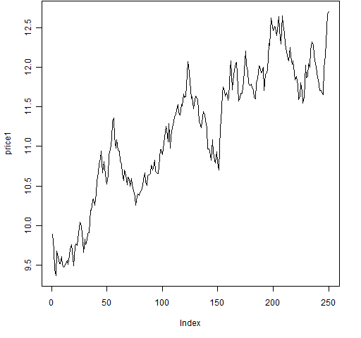Let’s make the novice mistake and perform a linear regression to get the trend for the prices:

> seq1 <- 1:250
> summary(lm(price1 ~ seq1)) # the novice mistake

Call:
lm(formula = price1 ~ seq1)

Residuals:
Min       1Q   Median       3Q      Max
-0.79084 -0.29531  0.00158  0.28625  0.91303

Coefficients:
Estimate Std. Error t value Pr(>|t|)
(Intercept) 9.8615883  0.0462913  213.03   <2e-16 ***
seq1        0.0105576  0.0003198   33.02   <2e-16 ***
---
Signif. codes:  0 ‘***’ 0.001 ‘**’ 0.01 ‘*’ 0.05 ‘.’ 0.1 ‘ ’ 1

Residual standard error: 0.3649 on 248 degrees of freedom
Multiple R-squared: 0.8147,     Adjusted R-squared: 0.8139
F-statistic:  1090 on 1 and 248 DF,  p-value: < 2.2e-16

Note that the coefficient for seq1 (the trend) is highly significant, as is (equivalently in this case) the overall regression.

Bootstrapping the regression

We can use the statistical bootstrap to see the variability of the trend coefficient.

> bootco1 <- numeric(1000)
> for(i in 1:1000) {
+    bsamp <- sample(250, 250, replace=TRUE)
+    bootco1[i] <- coef(lm(price1[bsamp] ~
+      seq1[bsamp]))[2] + }
> quantile(bootco1, c(.025, .975))
2.5%       97.5%
0.009885522 0.011224954

So the trend coefficient is very close to 0.01.

Multiple price regressions

We’ve looked at one example.  Let’s do the same thing several times to get a real feel for what is going on.

We could create more objects like price1, but the “R way” of doing this is to create a list where each component is like price1.

> rlist <- vector("list", 5)
> for(i in 1:5) rlist[[i]] <- rt(250, 6) / 100
> plist <- lapply(rlist, function(x) 10 * exp(cumsum(x)))

Above we have created 5 return vectors in a list, and then created a new list holding the 5 corresponding price vectors.

Now we bootstrap the trend coefficient for each price series:

> blist <- rep(list(numeric(1000)), 5)
> for(j in 1:1000) {
+    bsamp <- sample(250, 250, replace=TRUE)
+    for(i in 1:5) {
+       blist[[i]][j] <- coef(lm(plist[[i]][bsamp] +          ~ seq1[bsamp]))[2] +    }
+ }

A plot of the bootstrap distributions is then made:

> dlist <- lapply(blist, density)
> dx.range <- range(lapply(dlist, "[", "x"))
> dy.range <- range(lapply(dlist, "[", "y"))
> plot(0, 0, type="n", xlim=dx.range, ylim=dy.range,
+     xlab="Coefficient value", ylab="Density")
> for(i in 1:5) lines(dlist[[i]], col=i+1, lwd=2)

Figure 2: Bootstrap distributions of price trend coefficients.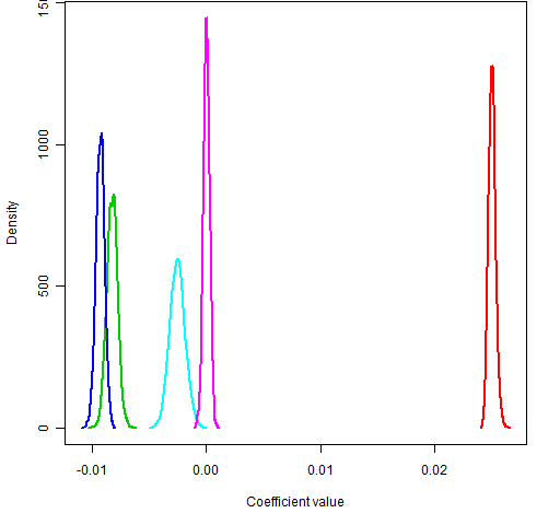

So we have used the exact same random generation method for five datasets and we get significantly different results from them.  Something has to be wrong.

But why?

In The tightrope of the random walk I imply that if a price series is a random walk, then the returns are uncorrelated.  That is, the returns are very much like a random sample.

The reality is that prices don’t exactly follow a random walk.  But they will be close enough that treating returns as uncorrelated is unlikely to lead you astray.

But prices (of the same asset across time) are correlated.  Very correlated.  If halfway through the year the price is higher than the starting price, then it is likely the final price of the year will be higher as well — even when there is no trend.

Variance

If we want a variance matrix, then we should also do our computation on returns and not prices.

Each of the five series that we generated were independent of each other, so they should be uncorrelated.  Here’s the variance we get for the price series:

> round(var(do.call("cbind", plist)), 2)[,1]  [,2]  [,3]  [,4]  [,5] [1,]  3.56 -1.17 -1.26 -0.39 -0.05[2,] -1.17  0.68  0.41  0.38  0.14[3,] -1.26  0.41  0.59  0.20  0.01[4,] -0.39  0.38  0.20  0.43  0.13[5,] -0.05  0.14  0.01  0.13  0.14

Alternatively we can compute the correlation matrix for the prices:

> round(cor(do.call("cbind", plist)), 3)[,1]   [,2]   [,3]   [,4]   [,5] [1,]  1.000 -0.753 -0.868 -0.311 -0.067[2,] -0.753  1.000  0.649  0.705  0.460[3,] -0.868  0.649  1.000  0.393  0.026[4,] -0.311  0.705  0.393  1.000  0.511[5,] -0.067  0.460  0.026  0.511  1.000

Here is the variance for the returns (in percent):

> round(var(do.call("cbind", rlist))*1e4, 2)[,1]  [,2]  [,3]  [,4]  [,5] [1,]  1.48  0.03  0.06  0.05 -0.04[2,]  0.03  1.57 -0.06  0.20  0.03[3,]  0.06 -0.06  1.80 -0.09  0.09[4,]  0.05  0.20 -0.09  1.52  0.06[5,] -0.04  0.03  0.09  0.06  1.42

This looks more like what we should expect: the diagonal elements are all very similar and the off-diagonal elements are reasonably close to zero.

Epilogue

Photo by H. Dickins via everystockphoto.com.