
Specific differences between Ledoit-Wolf and factor models
May 23, 2011
What can we learn about the difference in structure between a Ledoit-Wolf variance matrix and a corresponding factor model variance?
Previously
We’ve generated a set of random portfolios with constraints on the risk fractions of a Ledoit-Wolf variance matrix, and a corresponding set of random portfolios with risk fraction constraints from a statistical factor model. The two variance matrices use data up to the end of 2008 Q3. See posts:
In this post we use the risk fractions of the random portfolios to explore how the Ledoit-Wolf variance differs from the factor model.
Risk fractions
The key thing that drives this analysis is that we can get the risk fraction for each asset in the random portfolios both for the variance matrix that was used to do the constraints and for the other variance matrix.
Are there systematic differences between the risk fractions from the two variances? Could such differences highlight possible trouble spots?
In each set of random portfolios, we selected the risk fractions that were more than 2% (and per force less than 5%) for the variance matrix that was used to do the constraints, and then found the corresponding risk fractions from the other variance matrix. Figure 1 shows a scatter plot of all those risk fractions.
Figure 1: Selected risk fractions from the Ledoit-Wolf constrained portfolios (gold) and the factor model constrained portfolios (green).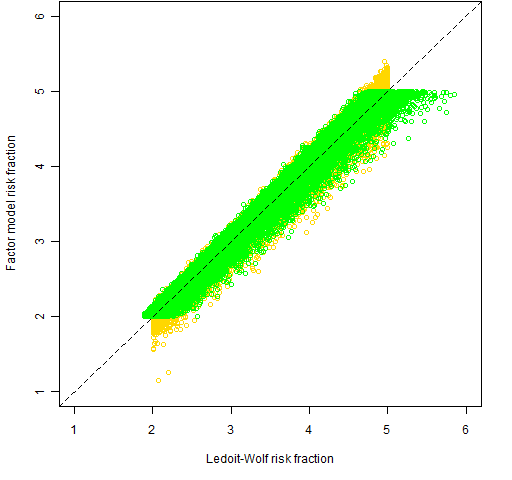 This shows a tendency for the Ledoit-Wolf risk fractions to be larger than the corresponding factor model risk fraction. Figure 2 displays this tendency in a different manner. This uses the same pairs of risk fractions as Figure 1, but the data is the ratio of the risk fraction from the non-constraining variance divided by the risk fraction from the constraining variance.
Figure 2: Boxplots of ratios of risk fractions — the constrained risk fractions are in the denominator. 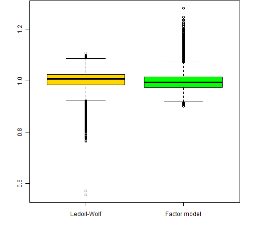 Both the Ledoit-Wolf risk fractions that have a ratio less than 0.6 are for ticker NEM. The stocks that have more than one factor model risk fraction with a ratio greater than 1.2 are CEG, WLP and EOG.
Correlations
We can look at the correlations embedded in the two variance matrices. Figure 3 shows the densities of the correlations.
Figure 3: Densities of the correlations from the Ledoit-Wolf estimate (gold) and the factor model (green). The vertical lines are the means. 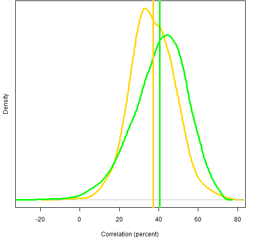 Notice that the factor model has more small correlations. A different perspective on this is Figure 4.
Figure 4: Comparison of Ledoit-Wolf and factor model correlations. 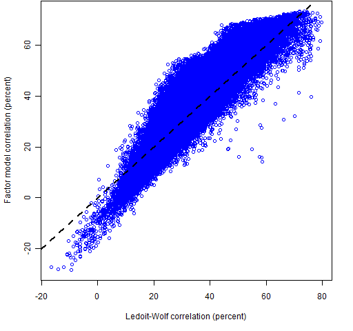 The spots where the factor model correlation is substantially smaller than the Ledoit-Wolf correlation may be problematic for the factor model. The correlations that are greater than 50% from Ledoit-Wolf but less than 20% from the factor model are:
AIG CEG
APOL DV
AET WLP
CI WLP
UNH WLP
Appendix R
Here we show the correlation part of the analysis. First is to get the unique correlations:
cor08Q3lw <- cov2cor(sp500.var08Q3)[lower.tri( sp500.var08Q3)]
cor08Q3fm <- cov2cor(sp500.fmvar08Q3)[lower.tri( sp500.fmvar08Q3)]
These use the inbuilt functions cov2cor (to change a variance matrix into a correlation matrix) and lower.tri (to get the lower triangle of values of a matrix).
From a computing point of view, the interesting part of the analysis is how to get the names of the variables for correlations that have specific characteristics:
outinds <- which(cov2cor(sp500.var08Q3) > .5 & cov2cor(sp500.fmvar08Q3) < .2, arr.ind=TRUE)
outindsr <- outinds[outinds[,1] < outinds[,2],]
outnams <- outindsr
outnams[] <- rownames(sp500.var08Q3)[outindsr]
The key trick is to use the which function with array index output. This gives us a two-column matrix. Next we cut the number of rows of this matrix in half by selecting the locations in the upper triangle. Finally we populate the locations in the matrix with asset names rather than numerical subscripts.
