
Risk fraction constraints and volatility
April 21, 2011
What is the effect on predicted and realized volatility of substituting risk fraction constraints for weight constraints?
Previously
This post depends on two previous blog posts:
The exact same sets of random portfolios are used in this post that were generated in the second of these.
Payoff
Figure 1 shows the volatility realized in Q4 of 2008 versus the predicted volatility at the beginning of the quarter for the 1000 random portfolios that constrained asset weights to no more than 5%. The correlation is 63%.
Figure 1: Predicted versus 2008 Q4 realized volatility for weight-constrained random portfolios.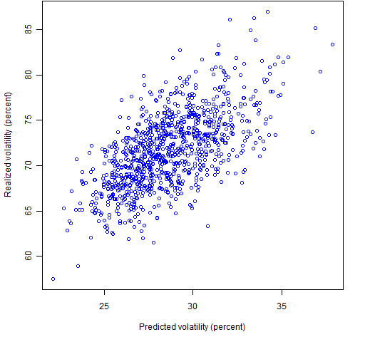
Figure 2: Predicted versus 2008 Q4 realized volatility for random portfolios with risk fraction constraints.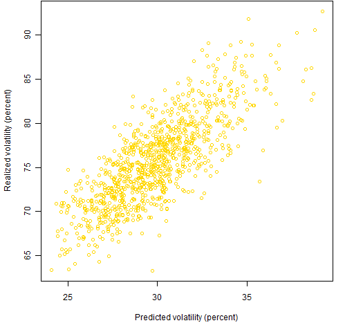
Figure 2 shows predicted versus realized volatility for the random portfolios that had risk fraction constrained to no more than 5%. The correlation here is a much better 79%.
If we were optimizing, the risk fraction constraints would probably give us better results. When we optimize, what we really care about is the ordering in terms of utility of the relevant portfolios. The relevant portfolios are those from which the random portfolios are a sample (that is, those obeying all the constraints). Generally the utility has expected returns as well as risk, but having risk ordered better should help order utility better.
Price
From the no-free-lunch department: We shouldn’t be surprised that there is a down-side to the risk fraction constraints. Figures 3 and 4 show the distribution of predicted and realized volatilities for the two sets of random portfolios.
Figure 3: Predicted volatility at the end of 2008 Q3 for random portfolios with weight constraints (blue line) and risk fraction constraints (gold line).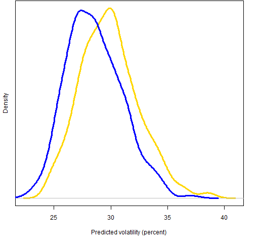
Figure 4: Realized volatility for 2008 Q4 for random portfolios with weight constraints (blue line) and risk fraction constraints (gold line).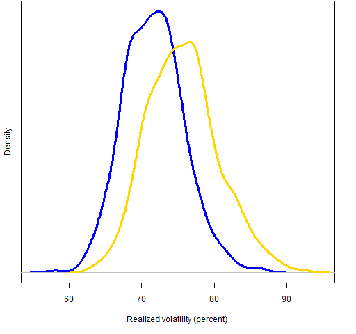
The risk fraction constraints are forcing more structure on the allocation of variance. This tends to induce a larger volatility for the portfolio.
I’m wondering how much the better optimization effect offsets the larger volatility effect.
Appendix R
The creation of the data that went into the plots above largely depends on functionality in Portfolio Probe. Here are the main R commands.
require(PortfolioProbe)
Recover the predicted volatilities of the portfolios:
rp.08Q3.rf05.pvol <- sqrt(252 * unlist(randport.eval(rp.08Q3.rf05, keep='var.values')))
rp.08Q3.w05.pvol <- sqrt(252 * unlist(randport.eval(rp.08Q3.w05, keep='var.values', additional.args=list(variance=sp500.var08Q3))))
Compute the valuation for each day during the quarter for the random portfolios. The result of each of the two commands below is a matrix with days in the rows and portfolios in the columns.
rp.08Q3.rf05.Q4val <- valuation(rp.08Q3.rf05, prices=as.matrix(sp500.closeok[440:504,]), collapse=TRUE)
rp.08Q3.w05.Q4val <- valuation(rp.08Q3.w05, prices=as.matrix(sp500.closeok[440:504,]), collapse=TRUE)
Get the realized volatility for the portfolios:
rp.08Q3.w05.Q4vol <- sqrt(252) * sd(diff(log(rp.08Q3.w05.Q4val)))
rp.08Q3.rf05.Q4vol <- sqrt(252) * sd(diff(log(rp.08Q3.rf05.Q4val)))
