
Realized beta and beta equal 1
August 30, 2011
What does beta look like in the out-of-sample period for the portfolios generated to have beta equal to 1?
In the comments Ian Priest wonders if the results in “The effect of beta equal 1” are due to a shift in beta from the estimation period to the out-of-sample period. (The current post will make more sense if you read that one first.)
Realized beta
Creating the betas for the stocks for the first half of 2011 (the out-of-sample period) is easy enough — it is just another regression. Figure 1 compares the stock betas for the two periods.
Figure 1: Estimates of beta for the constituents of the S&P 500 for 2011 H1 versus 2010. 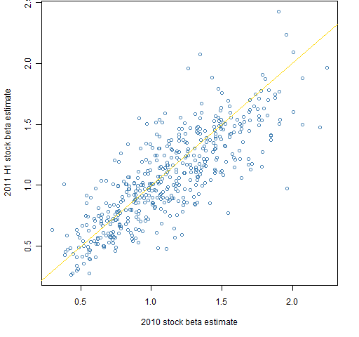
The realized betas for the portfolios are a bit trickier. They depend on the weights of assets in the portfolios, and the weights change throughout the period as the prices change. Figures 2 and 3 show the portfolio realized betas using either the weights at the start of the period or the weights at the end of the period.
Figure 2: Realized beta for portfolios of 20 assets using the portfolio weights either at the start or end of 2011 H1. 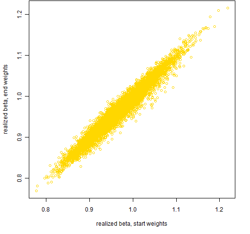
Figure 3: Realized beta for portfolios of 200 assets using the portfolio weights either at the start or end of 2011 H1. 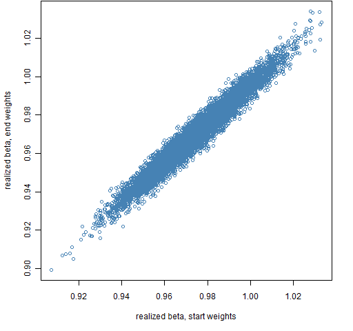
The surprise for me in these plots is how stable the portfolio betas are — that is, how close they remain to 1. Figure 6 of “4 and a half myths about beta in finance” indicates how variable stock betas can be.
As expected, using the weights at the mid-point tends to be a compromise between the weights at either end of the period.
Returns
Figures 4 and 5 show the portfolio returns versus the mid-point realized betas.
Figure 4: 2011 H1 returns for portfolios with 20 assets versus realized beta for the same period. 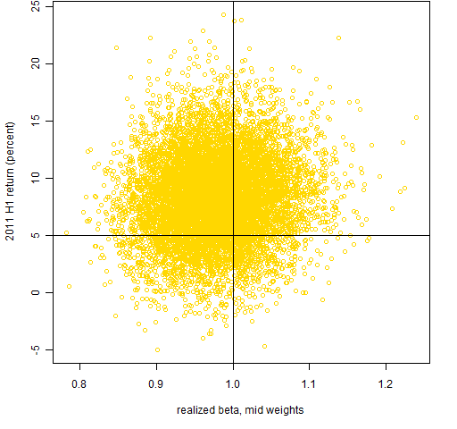
Figure 5: 2011 H1 returns for portfolios with 200 assets versus realized beta for the same period. 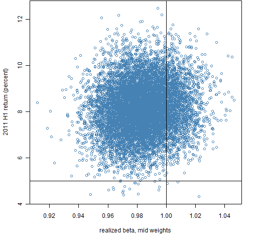
Appendix R
The first step is, of course, to estimate the betas for the new period:
spbeta2011H1 <- coef(lm(spcon2011H1 ~ spx2011H1))[2,]
The other step is to get the portfolio weights based on some set of prices and then multiply the weights by the corresponding betas and sum:
require(PortfolioProbe)
rbet1.spb1.20 <- unlist(lapply(valuation(ran.spb1.20, weight=TRUE, prices=spclose2011H1[1,]), function(x) sum(x * spbeta2011H1[names(x)])))
The valuation function in this case returns a list where each component is the weight vector of a random portfolio. A function to get the portfolio beta given the weights is then applied to each component of that list. Finally the resulting list of portfolio betas is simplified to a vector.

Nice blog.
Isn’t it that you are just showing here that a more or less equal weighted portfolio (I assume it’s close to what you get selecting 200 stocks at random from 500, slightly adjusting to get beta=1) does not perform like the SP500?
What about plot #5 with beta and return for an equal weighted portfolio of the 500 stocks? Does it hit in the centre of the cloud? That would suggest plotting next return 2011 H1 vs market cap.
Laurent,
Thanks for commenting. Your assumption is not quite right. The weights in these random portfolios are not at all close to equal weighting. I did do that exercise of doing close to equal weighting random portfolios with beta=1 — the distribution of returns was much tighter around the same center.
An equal weighting of all the stocks has a return of about 6.3% for 2011 H1, a beta of about 1.12 and a realized beta of about 1.06. So forcing the beta to be a little smaller pushes up the return quite a bit.