
Beta and expected returns
September 16, 2011
Some pictures to explore the reality of the theory that stocks with higher beta should have higher expected returns.
Figure 2 of “The effect of beta equal 1” shows the return-beta relationship as downward sloping. That’s a sample of size 1. In this post we add six more datapoints.
Data
The exact same betas of S&P 500 constituents are used as in “A brief history of S&P 500 beta”. Returns for the year following the point at which each set of betas became available are also used.
Pictures
Figures 1 through 6 each show returns versus beta. The blue line is the (default) lowess line through the data. The gold lines are lowess lines on 100 bootstraps of the data.
Figure 1: Returns versus beta estimate at start 2008. 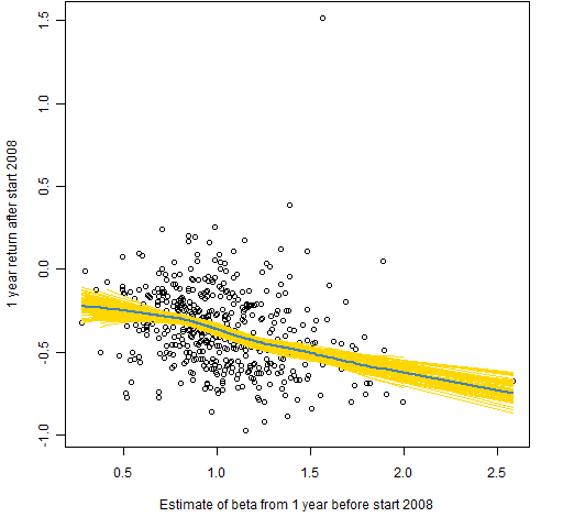
Figure 2: Returns versus beta estimate at mid 2008. 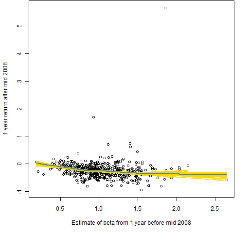
Figure 3: Returns versus beta estimate at start 2009. 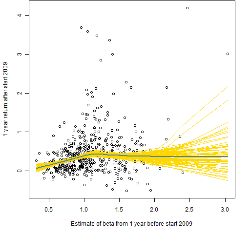
Figure 4: Returns versus beta estimate at mid 2009. 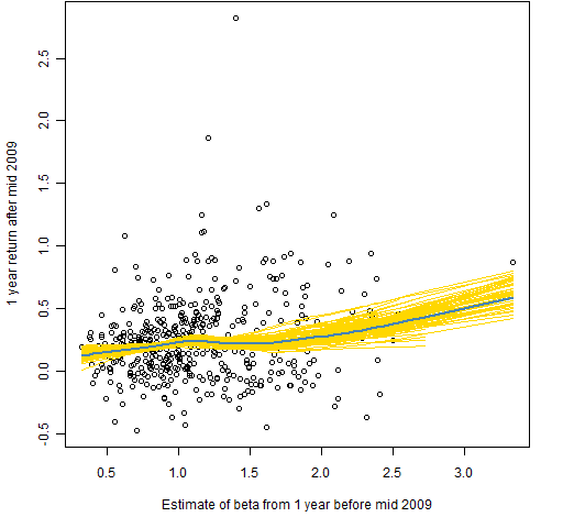
Figure 5: Returns versus beta estimate at start 2010. 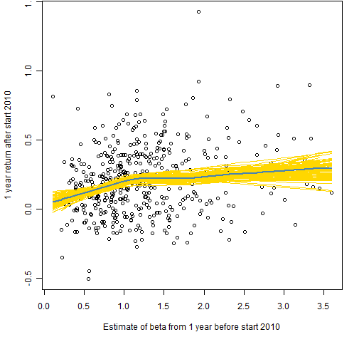
Figure 6: Returns versus beta estimate at mid 2010. 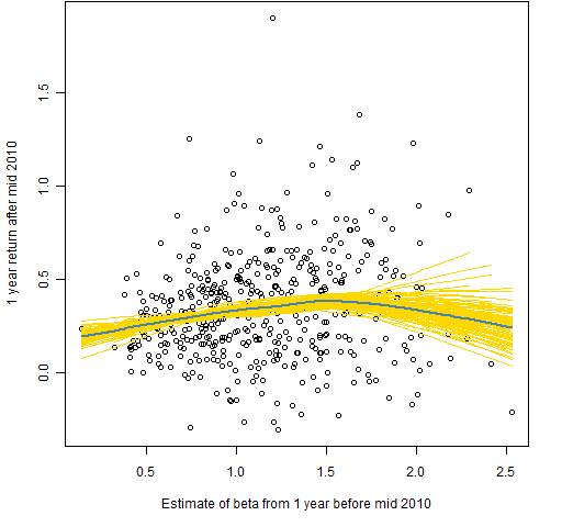
Discussion
Although Figures 1 and 2 are downward sloping, they are not evidence against the theory. Actually they support it — the low beta stocks tend to stay where they are, and the high beta stocks do as the market does (and perhaps more so).
It is the other four plots that are mainly of interest. The theory seems to hold periodically, but it is certainly not universally true. I suggest that this is a bit of evidence for low volatility investing (though beta should not be confused with volatility).
Appendix R
create annual returns
The first task is to create a matrix of annual returns starting at the appropriate places. This uses the objects created for “A brief history of S&P 500 beta”.
spannret <- spbetamat[,1:6]
spannret[] <- NA
for(i in 1:6) {
spannret[,i] <- colSums(spmat.ret[seq(sp.breakr[i+2], sp.breakr[i+4] - 1),-1])
}
spannret <- exp(spannret) - 1
summary(spannret)
Assigning NA to all the locations in the new matrix is not really necessary, but it is a safety measure. If something goes wrong in the overwriting process, we will know because we will see missing values.
plot
The figures are created with commands like:
pp.betareturn(1, boot=100, tofile=TRUE)
Here is the definition of pp.betareturn.
