Statistical factor models and Ledoit-Wolf shrinkage are competing methods for estimating variance matrices of returns.  So which is better?  This adds a data point for answering that question.

Previously

There are past blog posts on:

• the idea of variance matrices
• factor models of variance

The data in this post are from the blog posts:

• “Weight compared to risk fraction”
• “Risk fraction constraints and volatility”

Predictions

A Ledoit-Wolf variance estimate and a factor model estimate were both created on about a year of daily returns up to the end of the third quarter of 2008.  These are tested on two sets of random portfolios: one in which asset weights are constrained to be no more than 5%, and the other in which risk fractions are constrained to be no more than 5%.  The risk fraction constraints used the Ledoit-Wolf variance matrix.

Figures 1 and 2 show the predicted volatilities of the random portfolios.  At least to me, the predicted volatilities are amazingly similar between the two models.

Figure 1: Predicted volatilities at the end of 2008 Q3 for 1000 random portfolios with weights constrained to be less than 5%.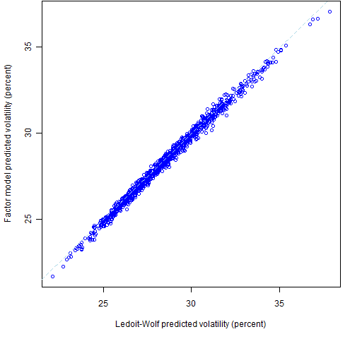

Figure 2: Predicted volatilities at the end of 2008 Q3 for 1000 random portfolios with Ledoit-Wolf risk fractions constrained to be less than 5%.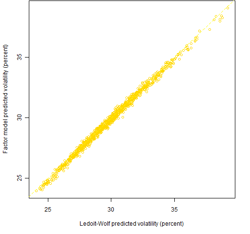

Predictions versus realized

We can compare the predicted volatilities to the realized volatilities of the portfolios for the fourth quarter of 2008.  The correlation (across portfolios) between predicted and realized volatility for the weight-constrained portfolios is 63.5% for Ledoit-Wolf and 63.3% for the factor model.  On the portfolios with risk fraction constraints the correlations are 78.8% for Ledoit-Wolf and 78.0% for the factor model.

Figures 3 and 4 use a bootstrap to show us how variable those numbers are.

Figure 3: Bootstrap distribution of correlation between Ledoit-Wolf predicted volatility and realized 2008 Q4 volatility for weight-constrained portfolios.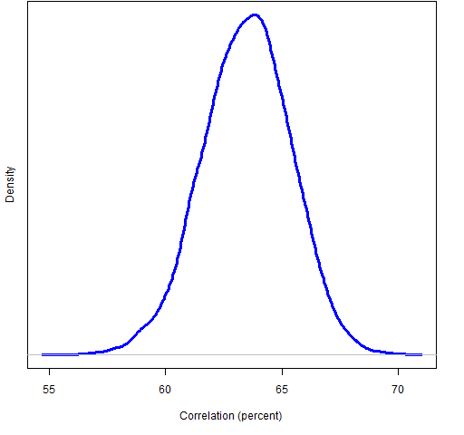

Figure 4: Bootstrap distribution of correlation between Ledoit-Wolf predicted volatility and realized 2008 Q4 volatility for portfolios with risk fraction constraints.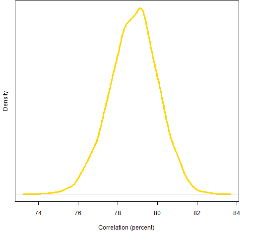

We can also explore how significant the differences in correlation are by bootstrapping.  To do this, the bootstrap samples need to be the same for the factor model as for Ledoit-Wolf.  Figures 5 and 6 show the distribution of correlation differences.

Figure 5: Difference in correlations for portfolios with weight constraints (positive difference means Ledoit-Wolf is better).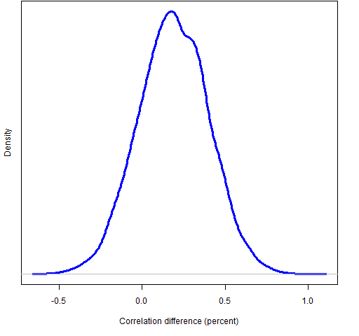

The fraction of bootstrap samples with negative differences is about 19% so there is no compelling reason to believe that Ledoit-Wolf is better in this instance.

Figure 6: Difference in correlations for portfolios with risk fraction constraints (positive difference means Ledoit-Wolf is better).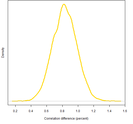

All of the differences are well above zero, but the superiority of Ledoit-Wolf in this instance may be an illusion.

Comments

The function that created the factor model has a selection criterion for the number of factors to use.  In this case it selected two factors.

It is possible that the Ledoit-Wolf estimate has an advantage over the factor model for the portfolios with risk fraction constraints because the constraints used the Ledoit-Wolf risk fractions.

Appendix R

The factor model is estimated with a function from the BurStFin package (available from the Burns Statistics website).

require(BurStFin)
sp500.fmvar08Q3 <- factor.model.stat(sp500.ret[seq(to=440, length=250),])

The predicted volatilities for the factor model can be computed:

require(PortfolioProbe)
rp.08Q3.w05.fmpvol <- sqrt(252 * unlist(randport.eval(rp.08Q3.w05, keep='var.values', additional.args=list(variance=sp500.fmvar08Q3))))

rp.08Q3.rf05.fmpvol <- sqrt(252 * unlist(randport.eval(rp.08Q3.rf05, keep='var.values', additional.args=list(variance=sp500.fmvar08Q3))))

Now all the ingredients are available to do the bootstrapping:

boot.w05.ledwolf <- numeric(10000)
boot.rf05.ledwolf <- numeric(10000)
boot.rf05.facmod <- numeric(10000)
boot.w05.facmod <- numeric(10000)

for(i in 1:10000) {
the.samp <- sample(1000, 1000, replace=TRUE)
boot.w05.ledwolf[i] <- cor(rp.08Q3.w05.pvol[the.samp], rp.08Q3.w05.Q4vol[the.samp])
boot.rf05.ledwolf[i] <- cor(rp.08Q3.rf05.pvol[the.samp], rp.08Q3.rf05.Q4vol[the.samp])
boot.w05.facmod[i] <- cor(rp.08Q3.w05.fmpvol[the.samp], rp.08Q3.w05.Q4vol[the.samp])
boot.rf05.facmod[i] <- cor(rp.08Q3.rf05.fmpvol[the.samp], rp.08Q3.rf05.Q4vol[the.samp])
}

Subscribe to the Portfolio Probe blog by Email