Winsorization replaces extreme data values with less extreme values.

But why

Extreme values sometimes have a big effect on statistical operations.  That effect is not necessarily a good effect.  One approach to the problem is to change the statistical operation — this is the field of robust statistics.

An alternative solution is to just change the data.  You can then use whatever statistical procedure you want.

In my experience in finance only mildly robust statistics (and hence only mildly winsorized data) are called for.  There seems to be a surprising amount of information in the tails of financial returns.

Trimming

There is an alternative to winsorization, which is just throwing out the extreme values.  That is called “trimming”.  The mean function in R has a trim argument so that you can easily get trimmed means:

> mean(c(1:10, 300))[1] 32.27273
> mean(c(1:10, 300), trim=.05)[1] 32.27273
> mean(c(1:10, 300), trim=.1)[1] 6

Trimming removes a certain fraction of the data from each tail.

Winsorizing — one way

One approach to winsorization is just to copy trimming, but replace the extreme values rather than throw them out.  Here is an R function that does this:
> winsor1
function (x, fraction=.05)
{
if(length(fraction) != 1 || fraction < 0 ||
fraction > 0.5) {
stop("bad value for 'fraction'")
}
lim <- quantile(x, probs=c(fraction, 1-fraction))
x[ x < lim[1] ] <- lim[1] x[ x > lim[2] ] <- lim[2] x
}

Figures 1 and 2 show this function in action.

Figure 1: The winsor1 function with some normally distributed data.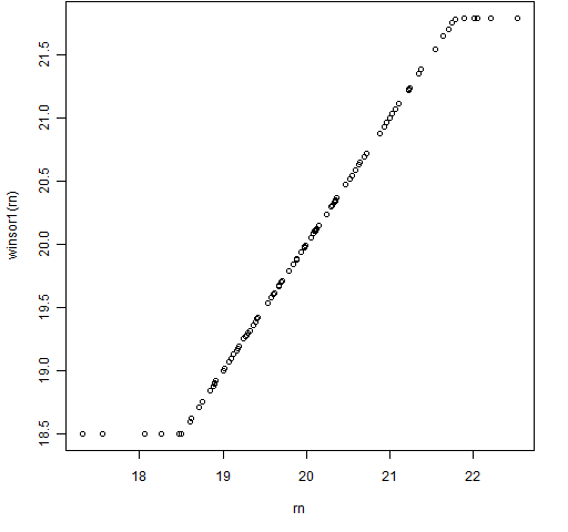
Figure 2: The winsor1 function with some Cauchy distributed data.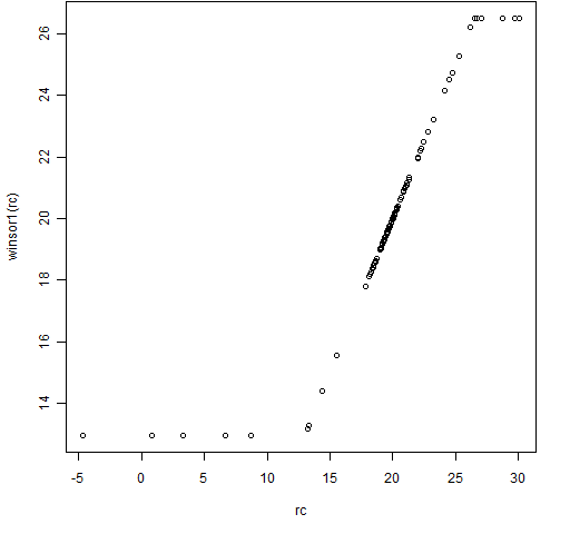

Winsorizing — another way

Another approach to winsorization is to try to just move the datapoints that are likely to be troublesome.  That is, only move data that are too far from the rest.  Here is such an R function:

> winsor2
function (x, multiple=3)
{
if(length(multiple) != 1 || multiple <= 0) {
stop("bad value for 'multiple'")
}
med <- median(x)
y <- x - med
sc <- mad(y, center=0) * multiple
y[ y > sc ] <- sc
y[ y < -sc ] <- -sc
y + med
}

Figures 3 and 4 show the results of this function using the same data as in Figures 1 and 2.

Figure 3: The winsor2 function with some normally distributed data.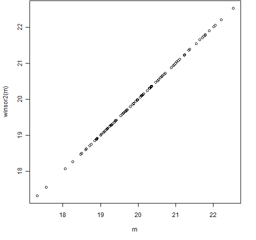
Figure 4: The winsor2 function with some Cauchy distributed data.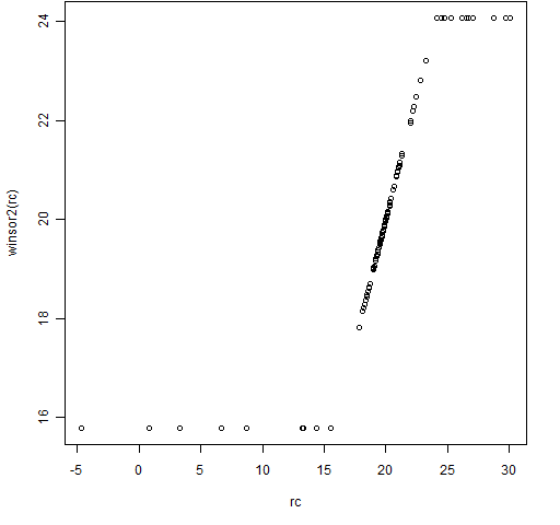

Comments

I think the second form of winsorization usually makes more sense.  In the examples the normal data are not changed at all by the second method and the Cauchy data look to be changed in a more logical way.

Production quality implementations of the R functions would probably include an na.rm argument to deal with missing values.

Subscribe to the Portfolio Probe blog by Email