
The indices understate the carnage
August 9, 2011
The first 6 trading days of August have been bad for the major indices, but how variable is that across portfolios?
To answer that, two sets of random portfolios were generated from the constituents of the S&P 500. The trading days are 2011 August 1 — 5 and 8.
The returns of the indices for this period were:
- S&P 500: -13.4%
- Dow Jones Industrials: -11.0%
- Nasdaq Composite: -14.5%
Small portfolios
The constraints for the small portfolios were:
- long-only
- exactly 20 assets in the portfolio
- weights between 1% and 10%
Figure 1 shows the distribution of the returns of 10,000 such portfolios.
Figure 1: Return distribution of portfolios of size 20 with the return of the Nasdaq Composite (black), the S&P 500 (blue) and Dow Jones Industrials (gold). 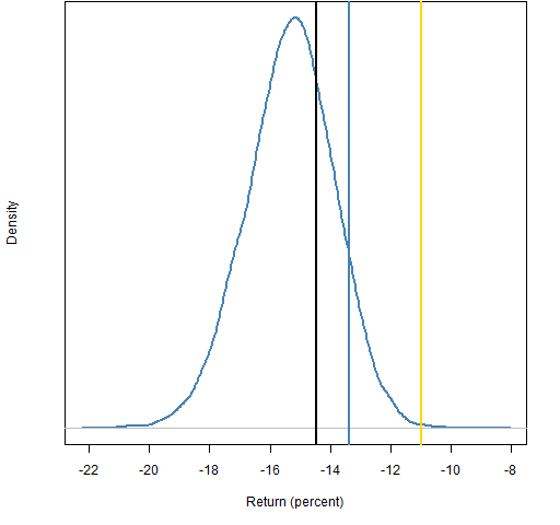
It appears that small stocks were hit harder than large caps.
Large portfolios
The constraints in this setting were:
- long-only
- exactly 200 assets in the portfolio
- weights between 0.1% and 5%
Figure 2 shows the returns of 10,000 portfolios with these constraints.
Figure 2: Return distribution of portfolios of size 200 with the return of the Nasdaq Composite (black), the S&P 500 (blue) and Dow Jones Industrials (gold).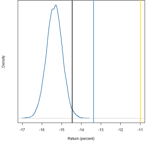
This is even more emphatic that the typical stock did worse than large caps.
Constituents
Figure 3: Distribution of S&P 500 constituents for the period.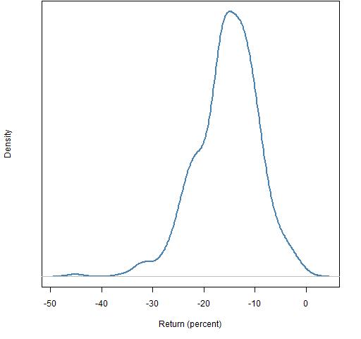
Appendix R
The data for this post was downloaded in the manner described in ‘On “Stock correlation has been rising”‘.
Once the data are in hand, there are four things to do:
Prepare the constraints
The minimum weight constraint requires a threshold constraint (a minimum weight constraint would be confusing in the light of long-short portfolios). In this case the easiest way of stating the appropriate threshold constraint is to give the amount of money the constraint represents via the positions argument. So we first create matrices suitable for that argument:
> sp.smpos <- cbind(-1, 1, -1, 1, 0, 0, 0, rep(.01, 490))
> sp.lgpos <- cbind(-1, 1, -1, 1, 0, 0, 0, rep(.001, 490))
This indicates that we actually have 490 constituents, not the full number.
generate the random portfolios
> require(PortfolioProbe)
> sp.rp20 <- random.portfolio(1e4, prices=sp500.close0808[1,], long.only=TRUE, gross=1e6, positions=sp.smpos*1e6, port.size=c(20,20), max.weight=.1)
> sp.rp200 <- random.portfolio(1e4, prices=sp500.close0808[1,], long.only=TRUE, gross=1e6, positions=sp.lgpos*1e6, port.size=c(200,200), max.weight=.05)
get the returns
> sp.rp20.ret <- pp.simpret(valuation(sp.rp20, prices=sp500.close0808[c(1,7),], collapse=TRUE))
> sp.rp200.ret <- pp.simpret(valuation(sp.rp200, prices=sp500.close0808[c(1,7),], collapse=TRUE))
plot the returns
> plot(density(sp.rp20.ret * 100))
> plot(density(sp.rp200.ret * 100))

[…] Indices understate the market carnage. (Portfolio Probe) […]