Why returns have a stable distribution

As “A tale of two returns” points out, the log return of a long period of time is the sum of the log returns of the shorter periods within the long period.

The log return over a year is the sum of the daily log returns in the year.  The log return over an hour is the sum of the minute log returns within the hour.

Returns have some distribution.  The set of distributions where their sums still have the same distribution are called stable distributions.  So log returns have a stable distribution.

Why returns have a normal distribution

There is a special distribution within the class of stable distributions called the normal distribution.  It is the only one that has a finite variance.

The Central Limit Theorem tells us conditions when the distribution of a sum is normal (to a good approximation).  Actually there is more than one Central Limit Theorem.  Figure 1 shows the single theorem idea, while Figure 2 shows the actual case.

Figure 1: Sketch of The Central Limit Theorem.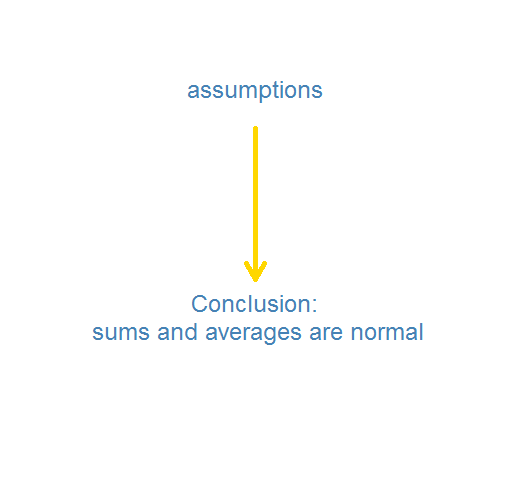

Figure 2: Sketch of The Central Limit Theorems.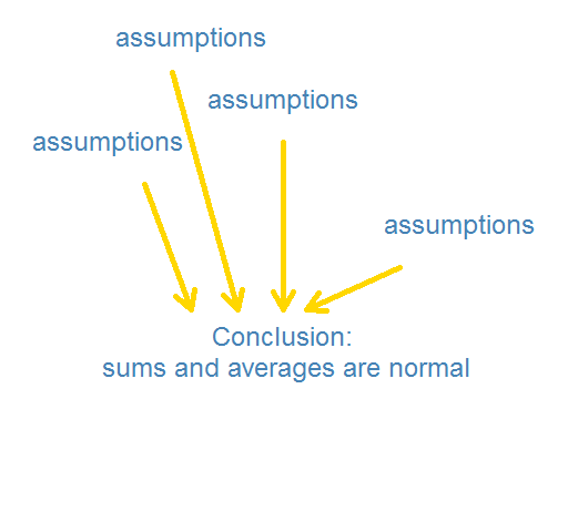

The commonality of the assumptions in Figure 2 can be summarized as:

• No giants among the peons
• Not too much dependence between the peons

Returns obey these criteria.  Therefore log returns have a normal distribution.

That applies to individual assets.  The returns of an index — which is the weighted average of a number of assets — has even more reason to be normal.  Even if the returns of the individual assets were not normal, the averaging over assets would mean that the index returns would be normal.

Data

The previous two sections are exquisitely reasoned.  So imagine my disappointment when people try to say that returns are not normally distributed.

Figure 3 shows the daily log returns of the S&P 500 over about six decades in the form of a normal QQplot.  Based on the variability of the middle half of the data, the most extreme returns we should have seen during that period was about 3%.  We’re not far off.

Figure 3: Normal QQplot of 6 decades of daily S&P 500 log returns. 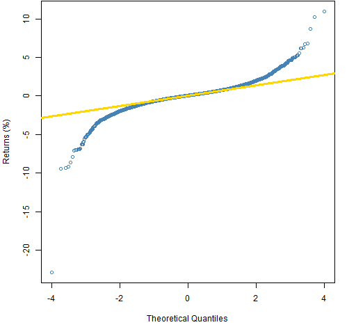A reason that the distribution would not be exactly normal is because of volatility clustering — that some periods have higher volatility than others.  We can look at the residuals from a garch model to remove that effect.  This is done in Figure 4.

Figure 4: Normal QQplot of 6 decades of daily GARCH residuals from S&P 500 log returns. 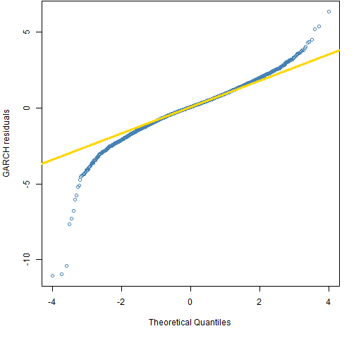Now that’s better, isn’t it?  If you think that volatility clustering negates the logic that leads us to the stable distribution conclusion, then, well, uh … think something else.

We don’t have to rely on pictures, we can do a statistical test.  Jarque-Bera tests normality by looking at the skewness and kurtosis.  The p-value for the test on the garch residuals is bigger than 10 to the minus 2800.  Somewhat smaller than the probability of winning a lottery — but people win lotteries all the time.

Discussion

If we were to consider the hypothetical possibility that returns are not normally distributed, how might that happen?

One way would be if returns across periods did depend on each other.  Perhaps if enough people did momentum trades in which they buy because the price has gone up, and sell because the price has gone down.

But of course markets don’t work like that.  People trade based on real information (and they evaluate that information without regard to how others value it).  News arrives and the market quickly adjusts to that new information.

If data seems to contradict logic, the only civilized thing to do is to stick to logic.

Epilogue

and if you think that you can tell a bigger tale
I swear to God you’d have to tell a lie…

from “Swordfishtrombone” by Tom Waits

Appendix R

qqplot

A simple version of Figure 3 is:

qqnorm(spxret)
qqline(spxret, col="gold")

garch estimate

The GARCH(1,1) model was estimated via:

require(tseries)

spxgar <- garch(spxret)

The QQplot for the residuals was created with:

qqnorm(spxgar$resid[-1])

The square brackets with negative 1 inside them removes the first element of the residual vector (because it is a missing value).

normality test

The tseries package also has the jarque.bera.test function.

> jarque.bera.test(spxgar$resid[-1])

Jarque Bera Test

data:  spxgar$resid[-1] X-squared = 12721.34, df = 2, p-value < 2.2e-16

We get the real p-value (as opposed to the wimpy cop-out of being less than 2.2e-16) with a slight bit of computing:

> pchisq(12721.34, df=2, lower.tail=FALSE, log.p=TRUE) / log(10)[1] -2762.404

Subscribe to the Portfolio Probe blog by Email