How good is the current opportunity to pick stocks relative to the past?

Idea

The more stocks act differently from each other relative to how volatile they are, the more opportunity there is to benefit by selecting stocks.  This post looks at a particular way of investigating that idea.

Data

Daily (log) returns of 442 large cap US stocks with histories back to the start of 2004 were used.

The ratio

Consider a window of returns over a certain period and of a certain universe of assets.  We can get a measure of the variability of these returns in two ways:

• find the standard deviation across the universe for each time point, and then average those numbers (variability across assets)
• average the returns at each time point and then get the standard deviation of those averages (variability across time)

The first thought for many people is that these should give the same number.  They don’t.

The bigger the first number is relative to the second, the more possibility there is to profitably select assets.  If the second is large relative to the first, then the market is volatile but all the assets tend to move together.

The “opportunity ratio” is the first number divided by the second.  Below are pictures of how the ratio changes over time for rolling windows of 200 days and 60 days.

Results

Figures 1 and 2 show the opportunity ratio through time.

Figure 1: 200-day rolling window of the opportunity ratio.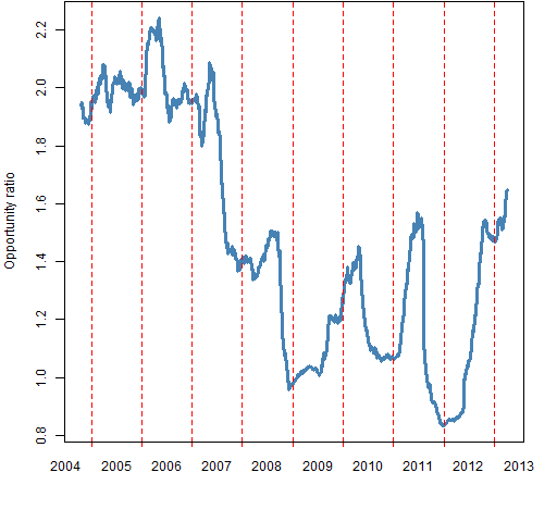

Figure 2: 60-day rolling window of the opportunity ratio. 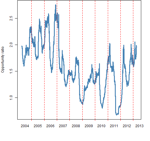These pictures show (at least) two things:

Almost always the ratio is bigger than 1.  This supports the view that “the market” is an over-simplification — these stocks have a tendency to march to their own drummer.

There is some hope that the ratio is recovering from the financial crisis.

Estimating variability

The final value for the 200-day ratio is 1.65, and 1.96 for the 60-day ratio.  The last day in the data is 2013 April 5.  We might like to know how variable these numbers are — they are, afterall, estimates based on data.

A common way of getting a sense of the variability of a statistic is to use the statistical bootstrap.  A complication here is that we want to account for variability due to both the time points and the assets.  That’s okay — we can do resampling on both of those simultaneously.

Figures 3 and 4 show the bootstrap distributions for the two final ratios.

Figure 3: bootstrap distribution of the opportunity ratio for the 200 days ending on 2013 April 5.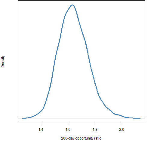

Figure 4: bootstrap distribution of the opportunity ratio for the 60 days ending on 2013 April 5.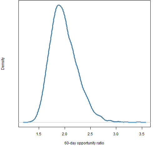

Most of the variability seems to come from resampling the days rather than the assets.  There are more assets which is probably at least part of the reason.

Summary

Stock-picking opportunity seems to be good relative to the rest of the post-crisis period.

This is a simple, but perhaps reasonable approach to exploring selection opportunity.

Appendix R

Computations were done in R.

compute the ratio

A function to compute a single ratio is:

pp.sdratioSingle <- function(retmat)
{
  # single computation of opportunity ratio

  # Placed in the public domain 2013 by Burns Statistics

  # Testing status: untested

  mean(apply(retmat, 1, sd)) / sd(rowMeans(retmat))
}

A function to compute rolling windows of the ratio is:

pp.sdratio <- function(retmat, window=200)
{
  # rolling window computation of opportunity ratio

  # Placed in the public domain 2013 by Burns Statistics

  # Testing status: untested

  averet <- rowMeans(retmat)
  vol <- rollapply(averet, FUN=sd, width=window, 
     align="right")
  daycross <- apply(retmat, 1, sd)
  cross <- rollapply(daycross, FUN=mean, width=window, 
     align="right")
  names(vol) <- names(cross)
  list(volatility=vol, cross.sd=cross, ratio=cross/vol, 
     call=match.call())
}

This latter function is used like:

opportun <- pp.sdratio(diff(log(univclose130406)))

time plot

The function used to create Figures 1 and 2 is pp.timeplot which you can put into your R session with:

source("https://www.portfolioprobe.com/R/blog/pp.timeplot.R")

bootstrap

A function that will return one matrix that has the original rows and/or columns bootstrapped is:

pp.matrixboot <- function(x, rows=TRUE, columns=TRUE)
{
  # bootstrap sampling on rows and/or columns of a matrix

  # Placed in the public domain 2013 by Burns Statistics

  # Testing status: untested

  dx <- dim(x)
  if(rows) {
    rsub <- sample(dx[1], dx[1], replace=TRUE)
  } else {
    rsub <- TRUE
  }
  if(columns) {
    csub <- sample(dx[2], dx[2], replace=TRUE)
  } else {
    csub <- TRUE
  }
  x[rsub, csub]
}

This was used like:

orboot200 <- orboot60 <- numeric(5000)
for(i in seq_along(orboot200)) {
  orboot200[i] <- pp.sdratioSingle(pp.matrixboot(lateret))
}