
More S&P 500 correlation
July 28, 2011
Here are some additions to the previous post on S&P 500 correlation.
Correlation distribution
Before we only looked at mean correlations. However, it is possible to see more of the distribution than just the mean. Figures 1 and 2 show several quantiles: 10%, 25%, 50%, 75%, 90%.
Figure 1: Quantiles of 50-day rolling correlation of S&P 500 constituents to the index. 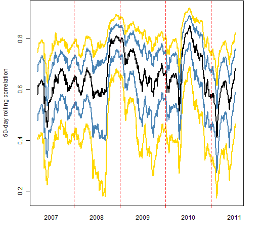 Figure 2: Quantiles of intra-constituent 50-day correlations.
 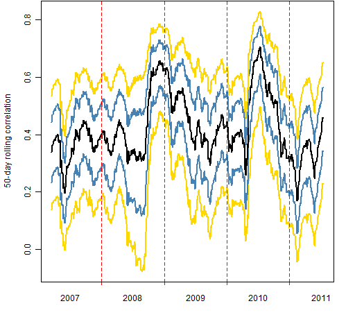 I don’t see anything special going on recently (this is still with data that ends July 15). Mid 2008 is interesting though: the small correlations got very small until Lehman came along.
Correlation uncertainty
Last time we used the statistical bootstrap to investigate variability. That was fine for thinking about the variability from constituents. However, it is reasonably unintuitive when looking at the variability due to different days.
Another approach is to look at what happens when we leave out one observation at a time. In statistical terminology this is the “jackknife” — it was used before the bootstrap came along.
Figure 3 shows the range of the 50 jackknifed results at each time point for the mean correlation among the constituents. We’re making a very small change here — dropping one day out of 50 — yet the result can move a non-trivial amount.
Figure 3: Leave-one-out range of mean intra-constituent 50-day correlations. 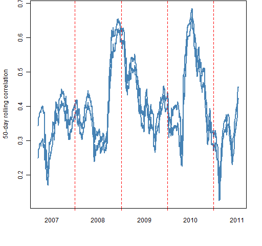 Figure 4 shows how the width of the jackknife range changes through time.
Figure 4: Width of the jackknife range for mean 50-day intra-constituent correlation. 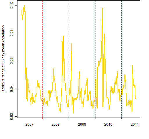
Appendix R
Two additional functions were written for this post. They are:
> pp.quan.const.cor
function (x, probs, window=50, index=1)
{
x <- x[, -index]
ans <- x[, 1:length(probs)]
colnames(ans) <- probs
ans[] <- NA
wseq <- (1-window):0
lt <- lower.tri(diag(ncol(x)), diag=FALSE)
for(i in window:nrow(x)) {
ans[i,] <- quantile(cor(x[wseq+i,])[lt], probs=probs)
}
ans[-1:(1-window),]
}
> pp.jackknife.const.cor
function (x, window=50, index=1)
{
x <- x[, -index]
ans <- x[, 1:2]
ans[] <- NA
wseq <- (1-window):0
lt <- lower.tri(diag(ncol(x)), diag=FALSE)
jknife <- numeric(window)
jseq <- 1:window
for(i in window:nrow(x)) {
xw <- x[wseq+i,]
jknife[] <- NA
for(j in jseq) {
jknife[j] <- mean(cor(xw[-j,])[lt])
}
ans[i,] <- range(jknife)
}
ans[-1:(1-window),]
}
Each of these is assuming that the first column of the data holds the index returns.
