For those who naturally compute portfolio returns correctly here are some lessons in how to do it wrong.

The data

Random portfolios were generated from constituents of the S&P 500 with constraints:

• long-only
• exactly 20 assets in the portfolio
• no more than 10% weight for any asset
• (just for fun) the sum of the 5 largest weights no more than 40%

1000 portfolios were generated at the beginning of 2008.  We then look at the results over the subsequent year.

These lessons should be considered an application of “A tale of two returns”.

Lesson 1

Multiply the weights times log returns of the assets, and compare with the actual log returns of the portfolio.  This is done in Figure 1.

Figure 1: Log portfolio returns versus weights times log returns. 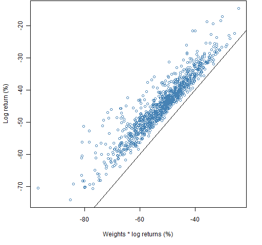Notice how the computed returns have a pleasing downward bias.

Lesson 2

We can really get some action if we compare the computation above with the simple returns of the portfolios, as in Figure 2.

Figure 2: Simple portfolio returns versus weights times log returns.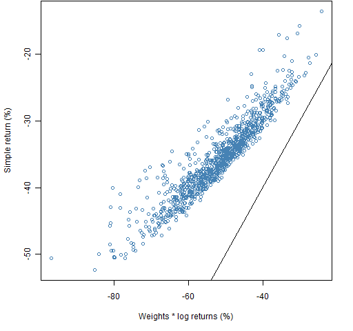

Lesson 3

Moving back towards subtlety, we can transform the weights times log returns to look like simple returns.  Figure 3 shows this.

Figure 3: Simple portfolio returns versus the transformation of weights times log returns.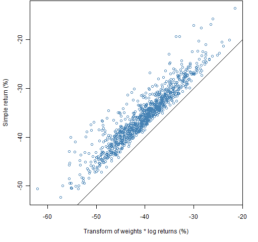

Avoid this

Multiplying simple returns times the weights and comparing that to the simple returns of the portfolios leads to a completely uninteresting plot, as in Figure 4.

Figure 4: Simple portfolio returns versus weights times simple returns.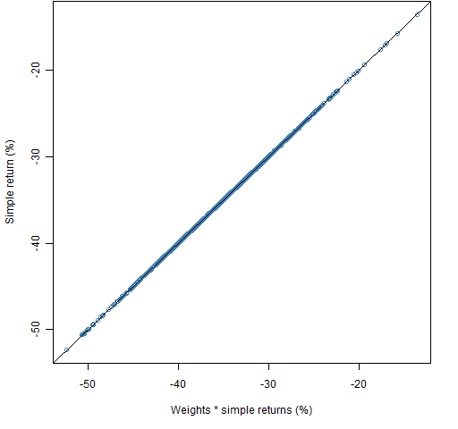

Epilogue

my Uncle Sol had a
chicken farm till the
skunks ate the chickens when

my Uncle Sol
had a skunk farm but
the skunks caught cold and
died and so

from “nobody loses all the time” by e. e. cummings

Appendix R

The computations exhibited here — except for the transformations — require the Portfolio Probe software.

require(PortfolioProbe)

generate random portfolios

rp08.20 <- random.portfolio(1000, prices=spmat.close[sp.breakr[3], -1], gross.value=1e6, long.only=TRUE, max.weight=.1, sum.weight=c("5"=.4), port.size=c(20,20))

portfolio returns

The following command returns a matrix of valuations with 254 rows (each trading day of 2008 plus 1) and 1000 columns (for each random portfolio).  That is because the prices argument is a matrix with 254 rows and columns corresponding to the assets.  If we were only interested in returns, prices could have been a matrix with only two rows — the first and last of what was given.

rp08.20.val <- valuation(rp08.20, prices=spmat.close[seq(sp.breakr[3],sp.breakr[5]),], collapse=TRUE)

rp08.20.rret <- pp.simpret(rp08.20.val[c(1,254),])

The actual computation in pp.simpret is:

x[2,] / x[1,] - 1

where x is a matrix.

weights times returns

The weight times return calculation can be done for the random portfolios via an indirect but labor-saving route.  The randport.eval function puts each random portfolio into the optimizer so we can recover components that the optimizer returns.  In this case we are interested in the expected return of the portfolio, which is named alpha.values in the optimizer output.

rp08.20.aret <- unlist(randport.eval(rp08.20, keep='alpha.values', additional.args=list(expected.return=ret2008)))

rp08.20.bret <- unlist(randport.eval(rp08.20, keep='alpha.values', additional.args=list(expected.return=exp(ret2008)-1)))

transformations

As we just saw above, a matrix of log returns can be transformed into simple returns with:

exp(ret2008)-1

The transformation in the other direction is:

log(simple.return.matrix + 1)

Subscribe to the Portfolio Probe blog by Email