
Bear hunting
December 6, 2010
When were there bear and bull markets in US stocks since 1950?
Smoothing
While we’d really like to estimate the expected return at each point in time, finding bear markets is ambitious enough. The plan starts by smoothing the daily returns through time, as in Figure 1.
Figure 1: Smoothed returns with a 4 year window.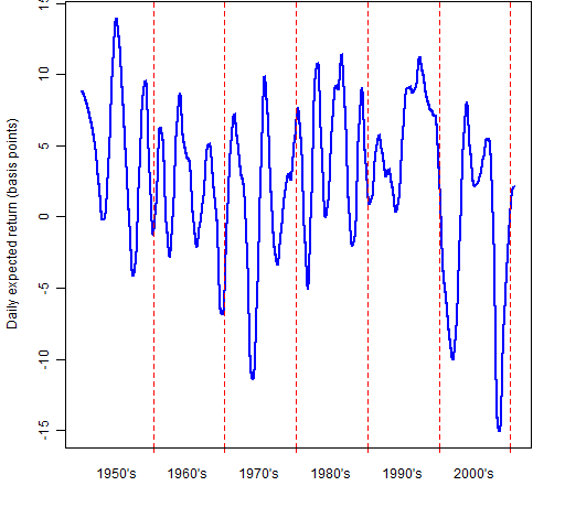
Note that for each time point we are using data in the future as well as in the past. This is a much easier task than predicting the return.
Figure 2: Smoothed returns with a half-year window.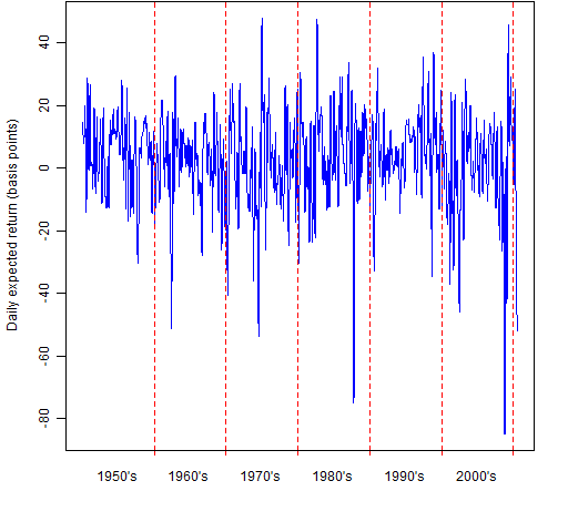 Of course both Figures 1 and 2 wiggle about. How are we to know what is significant wiggle, and what is just random wiggle? One thing to do is to smooth randomly permuted data. This will not have systematic good times and bad times. An example is in Figure 3.
Figure 3: Smoothed permuted returns with a half-year window.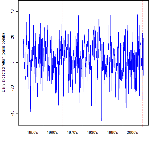 There is obviously structure in the returns because it is quite easy to tell which of Figures 2 and 3 is the real data. However, some of the structure that we see is from changing volatility. The mid-90’s were notorious for low volatility and this is definitely visible in Figure 2.
Calibrating noise
If there really are bull and bear markets, then those periods should have smooths that are outlying in the distribution of the smooths of randomly permuted data.
Figure 4: Densities of quarter-year window smooths of the returns (blue) and randomly permuted returns (green).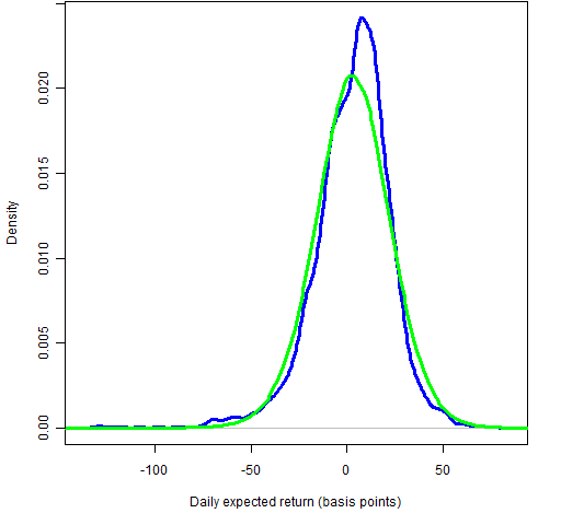 If we are to believe Figure 4, there were no bull markets during the 60 years and bear markets were rare and fairly subtle. We can use robust estimation in the smoothing process — Figure 5 shows the resulting densities.
Figure 5: Densities of quarter-year window robust smooths of the returns (blue) and randomly permuted returns (green).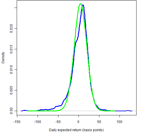
Figure 5 indicates more extensive bear markets, and also some possibility of bull markets. (By the way, the green lines in Figures 4 and 5 are much smoother than the blue lines because they are estimated with 100 times more data.)
Bear times
Four different smoothing windows were used: quarter-year, half-year, year, 4 years. Each of these were used with standard estimation and robust estimation. We don’t know which of these is best. But for each point in time we can plot how many of these 8 thought a bear market was on.
Figure 6: Count of models in bear market. 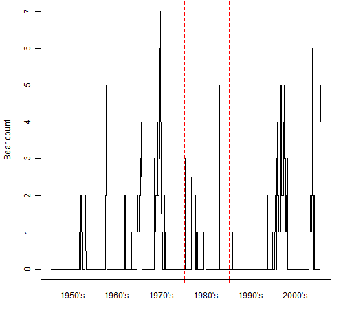 For each of the 8 models an arbitrary cutoff was established from inspecting the density plots like Figures 4 and 5.
Questions
This is far from a polished analysis. I have a couple ideas of how to make it better. What are your ideas?
Is there any way to know how smooth the expected return curve really is?
Some days you gets the bear, and some days the bear gets you. Which is this?
Appendix R
The smoother used was loess and the robust smooths used family="symmetric".
All of the data and functions used in the analysis are available.
In particular the function that highlights decades (and alternatively years) is a public domain function called pp.timeplot.
You can get the S&P data (spxdf and spxret) into your R session with:
> load(url('https://www.portfolioprobe.com/R/blog/bearspx.rda'))
You can get the functions (including pp.timeplot and functions to create the figures) with:
> source('https://www.portfolioprobe.com/R/blog/bearhunt.R')
The commands to recreate the analysis are in bearhunt.Rscript. Once these commands have been done, then you can use the plotting functions (starting with a capital P) to reproduce the figures.

[…] This post was mentioned on Twitter by Massimo Morelli, Patrick Burns. Patrick Burns said: Bear hunting http://bit.ly/epyCYw when did the US #stockmarket have bull and bear markets since 1950? #rstats […]