
Again with variability of long-short decile tests
December 6, 2012
A simpler approach to producing the variability.
Previously
The post “Variability in long-short decile strategy tests” proposed a way of assessing the variability of strategy tests in which a long-short portfolio is created by equally weighting the top and bottom deciles.
Improved idea
Joe Mezrich suggests maintaining equal weights but bootstrapping the assets within the deciles. For me that passes the jealousy test — why didn’t I think of that?
It eliminates the arbitrariness of the selection of the range of weights to use in the previous method.
Figure 1 shows the variability of 1000 bootstrap paths for the MACD signal that the previous post used.
Figure 1: Efficacy of MACD via long-short deciles with bootstrapped equal weights. 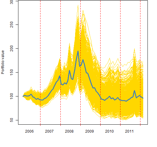 The bootstrap variability is bigger than the biggest of the variabilities investigated previously.
Appendix R
The function to do the bootstrapping is a very mildly revised version of the function that does the random weighting.
pp.decileTestBoot <-
  function(signal, prices, trials=1000, groups=10)
  {
    # R function to test a signal
    # via long-short deciles
    # and bootstrapping the deciles

    # put in the public domain 2012 by Burns Statistics

    # testing status:
    # seems to work

    stopifnot(all(dim(signal) == dim(prices)),
              length(groups) == 1,
              identical(sort(colnames(signal)),
              sort(colnames(prices))))

    ntimes <- nrow(prices)
    eqwtval <- rep(NA, ntimes)
    names(eqwtval) <- rownames(prices)
    randwtval <- array(NA, c(length(eqwtval), trials),
                       list(names(eqwtval), NULL))
    uret <- tail(prices, -1) / head(prices, -1) - 1
    randwtval[1,] <- eqwtval[1] <- 100

    nside <- round(ncol(prices) / groups)

    if(trials) {
      tseq <- 1:trials
      t.eret <- numeric(trials)
    }

    for(i in 1:(ntimes-1)) {
      tb <- pp.topBottom(signal[i, ], n=nside)
      botret <- uret[i, tb$bottom]
      topret <- uret[i, tb$top]
      this.eret <- mean(topret) - mean(botret)
      eqwtval[i+1] <- eqwtval[i] * (1 + this.eret)
      if(trials) {
        for(j in tseq) {
          t.eret[j] <- mean(sample(topret, nside,
            replace=TRUE)) - mean(sample(botret,
            nside, replace=TRUE))
        }
        randwtval[i+1, ] <- randwtval[i, ] *
            (1 + t.eret)
      }
    }
    ans <- list(equal.weight=eqwtval,
        random.weight=randwtval, nside=nside,
        call=match.call())
    class(ans) <- "SignalTest"
    ans
  }

[…] ← Popular posts 2012 November Again with variability of long-short decile tests → […]