
A brief history of S&P 500 beta
September 8, 2011
Data
The data are daily returns starting at the beginning of 2007. There are 477 stocks for which there is full and seemingly reliable data.
Estimation
The betas are all estimated on one year of data.
The times that identify the betas mark the point at which the estimate would become available. So the betas identified by “start 2008” use data from 2007; and betas identified by “mid 2008” use data from Q3 and Q4 of 2007 plus Q1 and Q2 of 2008.
Results
Figure 1 shows the behavior over time of all of the beta estimates.
Figure 1: All betas at all times. 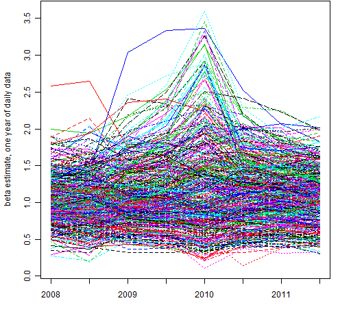 The stock that starts out with a beta estimate of about 2.6 (red line) is ETFC.
Figure 2 extracts the 20 stocks that exhibited the most volatility in their beta estimates over the 8 time points.
Figure 2: Betas exhibiting the most volatility through time. 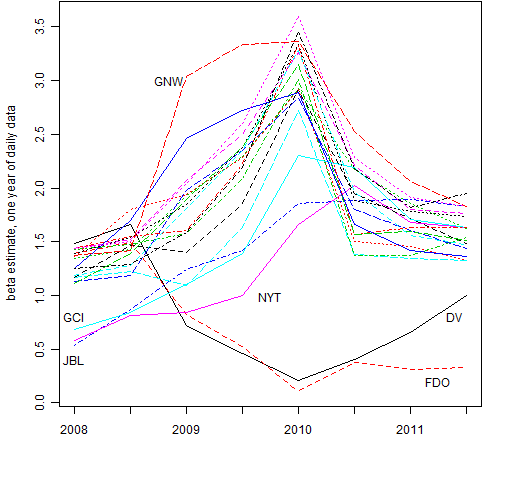 There are three groups visible:
- start low and go high
- start high and go low
- high and go very high in the middle
The tickers for the time marked 2010 (that is, using data from 2009) in Figure 2 are (from highest to lowest): LNC, HIG, GNW, FITB, HBAN, PRU, PFG, BAC, STT, HST, ZION, C, XL, PLD, PNC, GCI, JBL, NYT, DV, FDO.
Figure 3 shows the scatter of the first set of betas versus the last set. As would be expected, this is the pair with the lowest correlation.
Figure 3: Mid 2011 betas versus start 2008 betas. 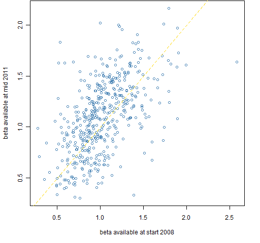
Appendix R
The creation of the original data can be seen at ‘On “Stock correlation has been rising”‘. There was then some minor data manipulation: create a matrix (rather than an xts object) with the index as the first column, and create a numeric vector (sp.breaks) that gives the break points for the year and half-year locations.
estimate betas
This involves creating a matrix to hold the beta estimates, and then filling that matrix via a for loop.
spbetamat <- array(NA, c(477, 8), list(colnames(spmat.close)[-1], names(sp.breaks)[-1:-2]))
for(i in 1:8) {
t.select <- seq(sp.breaks[i], sp.breaks[i+2] - 1)
spbetamat[, i] <- coef(lm(spmat.ret[t.select, -1] ~ spmat.ret[t.select, 1]))[2,]
}
plot
Figure 1 is created by:
matplot(t(spbetamat), type='l', xaxt='n', ylab="beta estimate, one year of daily data")
axis(1, at=1:8, labels=c("2008", "", "2009", "", "2010", "", "2011", ""))
get tickers
The list of tickers in Figure 2 was created with:
spbetavol <- sd(t(spbetamat)) jjhv <- names(tail(sort(spbetavol), 20)) jjbhv <- spbetamat[jjhv,] paste(rev(rownames(jjbhv[order(jjbhv[,5]),])), collapse=", ")
The result of the final command was then copied and pasted.

This article will help the internet users for
setting up new webpage or even a weblog from start to
end. finance-courses.com like best example!