Constraining the maximum asset-portfolio correlation gave bigger returns and smaller volatility.

Previously

“Portfolio diversity” introduced the topic of asset-portfolio correlations.  It also generated four sets of long-only random portfolios as of the start of 2011 using constituents of the S&P 500:

1. exactly 20 names, weights between 1% and 10%
2. exactly 20 names, maximum asset-portfolio correlation of 60%
3. exactly 200 names, weights between 0.1% and 1%
4. exactly 200 names, maximum asset-portfolio correlation of 60%

Here we see how those random portfolios performed during 2011.

2011 returns

Figures 1 and 2 show the distributions of the returns during the year.  The correlation constraint added substantial return for the year.

Figure 1: Distribution of 2011 returns of 20-name random portfolios: weight-constrained (gold) and correlation-constrained (blue).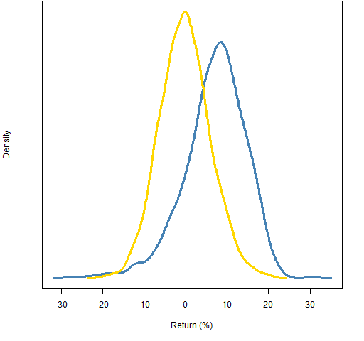

Figure 2: Distribution of 2011 returns of 200-name random portfolios: weight-constrained (gold) and correlation-constrained (blue).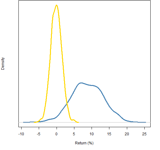

2011 realized volatility

The low correlation portfolios are also — in general — low volatility.  Perhaps that is the explanation of the high returns?

Figure 3: Distribution of 2011 realized volatility of 20-name random portfolios: weight-constrained (gold) and correlation-constrained (blue).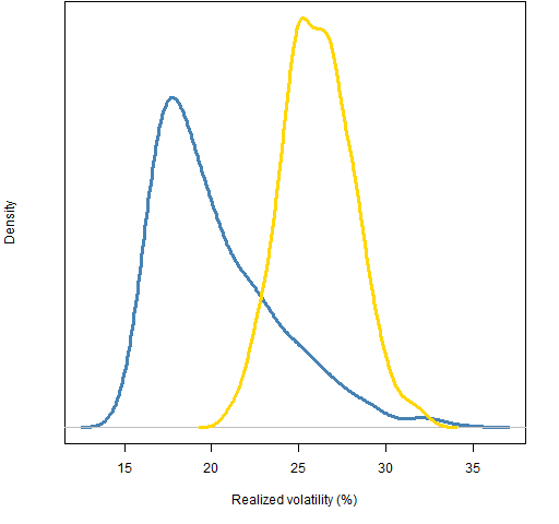

Figure 4: Distribution of 2011 realized volatility of 200-name random portfolios: weight-constrained (gold) and correlation-constrained (blue).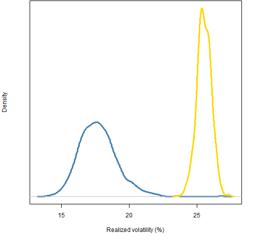

2011 information ratio

Figure 5: Distribution of 2011 information ratio of 20-name random portfolios: weight-constrained (gold) and correlation-constrained (blue).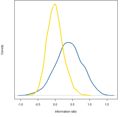

Figure 6: Distribution of 2011 information ratio of 200-name random portfolios: weight-constrained (gold) and correlation-constrained (blue).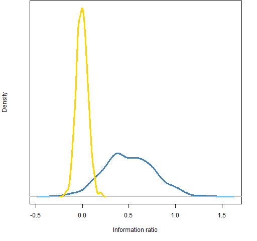

Summary

Adding the correlation constraint at the start of 2011 would have been quite useful.  I doubt that it is a magic bullet though.

Appendix R

The commands to generate the random portfolios were given in “Portfolio diversity”.

portfolio returns

The returns for the full year can be computed by giving valuation a two-row price matrix that has the first and last prices for the period.

> require(PortfolioProbe)
> divrp.20w.ret11 <- valuation(divrp.20w,
+    sp5.close11[c(1,253),], returns='simple')

portfolio volatilities

Computing the volatilities is only slightly more complicated.  We get the daily returns for the portfolios and then compute the standard deviation on the returns for each portfolio.

> divrp.20w.vol11 <- 100 * sqrt(252) * apply(valuation(
+    divrp.20w, sp5.close11, returns='simple'), 2, sd)

 

Subscribe to the Portfolio Probe blog by Email