
A bit of analysis of the Dow golden cross
April 16, 2011
I’d never heard of the golden cross before a few minutes ago. But The Reformed Broker talked about it. He lists some data that just ached to be thrown into a statistical bootstrap in R. So here it is.
Joshua informs us that a golden cross is when the 50-day moving average crosses above the 200-day moving average.
The bootstraps
We see just one average return for each time period: 2.4% for 1 month, 2.1% for 2 months and so on. But the data tell us more that just that. The idea of the bootstrap is to create a large number of alternative histories (I did 10,000) and see what distribution results over those histories. Figures 1 through 4 show the distributions.
Figure 1: Bootstrap distribution of 1-month Dow golden cross (vertical line represents the data mean).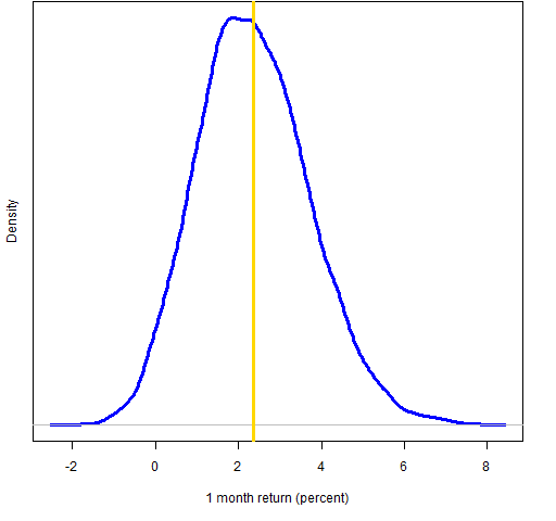
Figure 2: Bootstrap distribution of 2-month Dow golden cross (vertical line represents the data mean).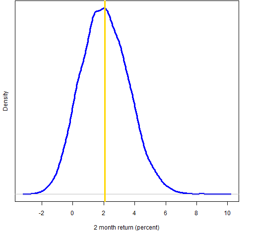
Figure 3: Bootstrap distribution of 3-month Dow golden cross (vertical line represents the data mean).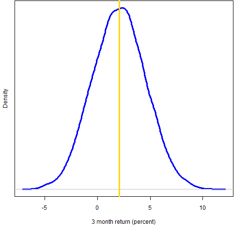
Figure 4: Bootstrap distribution of 6-month Dow golden cross (vertical line represents the data mean).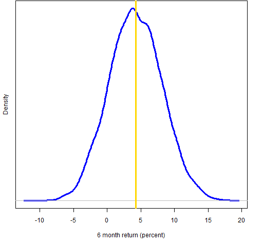
According to the bootstrap distributions there is about a 3% chance of a negative 1-month return, 8% for 2 months, 21% for 3 months and 14% for 6 months.
Appendix R
First is the code for getting the data into R. (Here are hints for beginning R.)
cg.1m <- c(2.6, 1.8, 0.9, 0.4, 6.4, -2.6, -2.9, 8.1, -.1, -.8, 12.1)
cg.2m <- c(7.5, 1.7, -1.3, -.7, 5.8, -2.4, -3.7, 7.1, -1.0, -2.6, 12.4)
cg.3m <- c(8.8, 3.3, -.1, -4.4, 12.7, -9.9, -8.4, 11.0, -1.5, -3.5, 14.8)
cg.6m <- c(-11.8, 6.1, 3.4, 4.3, 23.5, -4.2, -18.3, 14.4, 3.1, .4, 25.9)
Below is the code to do the four bootstraps:
cg.1mb <- numeric(10000)
cg.2mb <- numeric(10000)
cg.3mb <- numeric(10000)
cg.6mb <- numeric(10000)
for(i in 1:10000) cg.1mb[i] <- mean(cg.1m[sample(11,11, replace=TRUE)])
for(i in 1:10000) cg.2mb[i] <- mean(cg.2m[sample(11,11, replace=TRUE)])
for(i in 1:10000) cg.3mb[i] <- mean(cg.3m[sample(11,11, replace=TRUE)])
for(i in 1:10000) cg.6mb[i] <- mean(cg.6m[sample(11,11, replace=TRUE)])
Finally, here is the code to produce Figure 1:
plot(density(cg.1mb), lwd=3, col="blue", ylab="", main="",
xlab="1 month return (percent)", yaxt="n")
mtext("Density", side=2, line=1)
abline(v=mean(cg.1m), lwd=3, col="gold")
If you were making the plot just for yourself, you could do something like:
plot(density(cg.1mb))
abline(v=mean(cg.1m))

[…] look at statistics behind Dow “golden crosses.” (Portfolio Probe, The Reformed […]
hey, thanks for taking my post a step further, interesting stuff although some of it is a bit beyond me
jb
Josh,
My pleasure. The idea is very simple, and it is easy to think that it must be more complicated than it actually is.
Pat,
I really like your blog and your burns-stat.com site. I’ve learned a lot.
This problem is like any “indicator” type problem where I can’t tell how useful the scheme really is. In other words, the 50-day versus 200-day “Golden Cross” came from many people testing multiple n-day averages until they found and reported the best combination. So, how do you calculate a p-value or t-stat for this type of “Multiple Comparison” problem?
Here’s a similar situation that was described in the following paper (Dangers of Data-Driven Inference:The Case of Calendar Effects in Stock Returns):
http://citeseerx.ist.psu.edu/viewdoc/download?doi=10.1.1.12.1040&rep=rep1&type=pdf
In the paper, they were able to come up with a “Universe of Calendar Effects” of 9,452 rules (and a reduced set of 244 rules) to generate the statistics. In the “Golden Cross” scheme, can you think of a way to put a number to the “Universe of Golden Cross Effects”, and then look at the various p-value, t-stat, or whatever stats apply?
Thanks,
Bill
Bill,
That is a wonderful question to which I don’t have a good answer. Or pretty much any answer.
There is one good sign in that it is 50 and 200 as opposed to something like 47 and 213. On the other hand it is not 1 quarter and 1 year. There is a universe of crosses from which these data were selected. We can probably get a reasonable estimate of the size of that universe. Though it is not entirely clear to me how to go about adjusting for that.
But there is a much bigger universe. If none of the crosses looked interesting, then that table of data would be populated from some other scheme. I don’t think we have any hope of estimating the size of this larger universe.