How variable are garch predictions?
Previously
There have been several posts on garch, in particular:
Both of these posts speak about the two common prediction targets:
- prediction (of volatility) at the individual times (usually days)
- term structure prediction — the average volatility from the start to the time in question
It will be the latter that is investigated here.
Data and models
Daily log returns of the S&P 500 are used as the example. The latest data is from 2013 March 14.
There are four garch models that are investigated:
- component model with the t distribution
- component model with the normal distribution
- garch(1,1) with the t distribution
- garch(1,1) with the normal distribution
Figure 1 shows the volatility term structure estimated with each of the four models using 2000 daily returns.
Figure 1: Volatility term structure estimated with 2000 returns of component-t (blue), component-normal (green), garch(1,1)-t (gold) and garch(1,1)-normal (black). 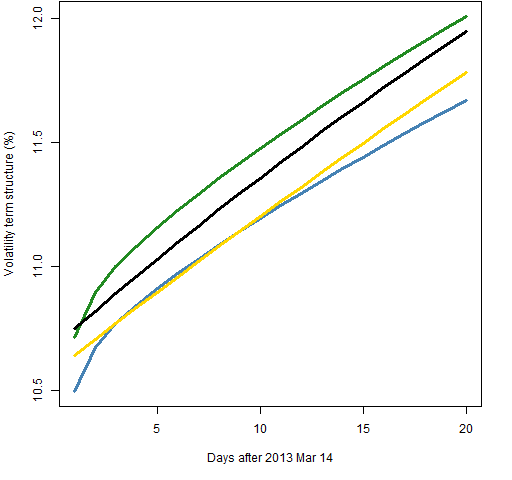
The more flexible prediction of the component model is evident. The distributional assumption does make a difference.
Method
Figure 1 shows variability between models, but let’s consider variability from a single model. Given a specific model, we get the parameter values for that model using the data. There is estimation error in those parameters. We get different predictions with different parameter values.
Variability is shown by doing: 200 series of the same length as the data were simulated with the estimated parameter values. So we know the true parameter values for those simulated series. Then the model is fit on each of the simulated series — the result is parameter values that are not the same as the true values. Finally predictions are produced from the real data using the newly estimated parameters.
In the plots below the prediction using the estimated parameters is in blue while the predictions using the parameters found from the simulated data are in gold.
Results
Figure 2 shows the prediction variability using 2000 returns and the component model with a t distribution. Figure 3 is for the component with normal model, Figure 4 the garch(1,1) with the t, and Figure 5 is for the garch(1,1) with the normal.
Figure 2: Volatility term structure variability for the component model with t distribution and 2000 returns. 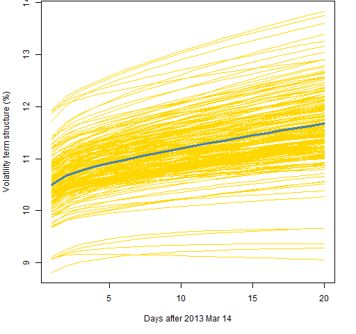
Figure 3: Volatility term structure variability for the component model with normal distribution and 2000 returns. 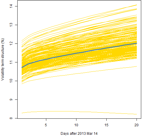
Figure 4: Volatility term structure variability for the garch(1,1) with t distribution and 2000 returns. 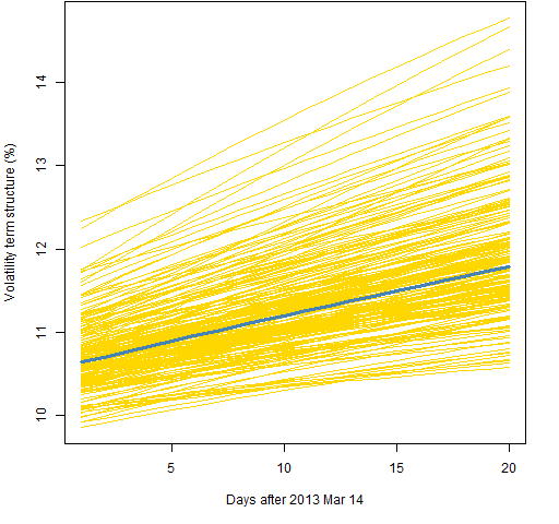
Figure 5: Volatility term structure variability for the garch(1,1) with normal distribution and 2000 returns. 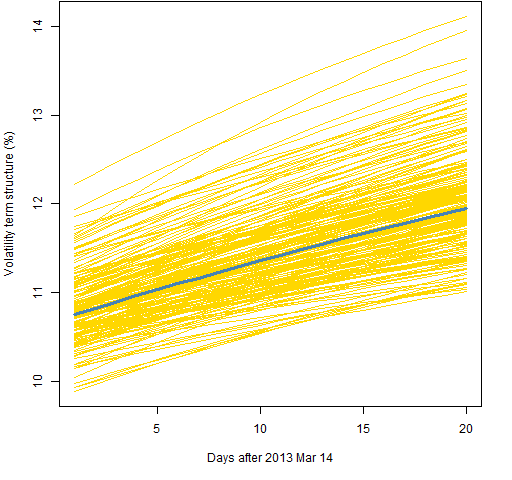 Figures 6, 7 and 8 all use the component model with the t distribution, like Figure 2. The difference is the amount of data used.
Figure 6: Volatility term structure variability for the component model with t distribution and 5000 returns. 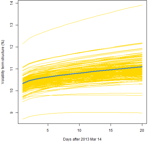
Figure 7: Volatility term structure variability for the component model with t distribution and 1000 returns. 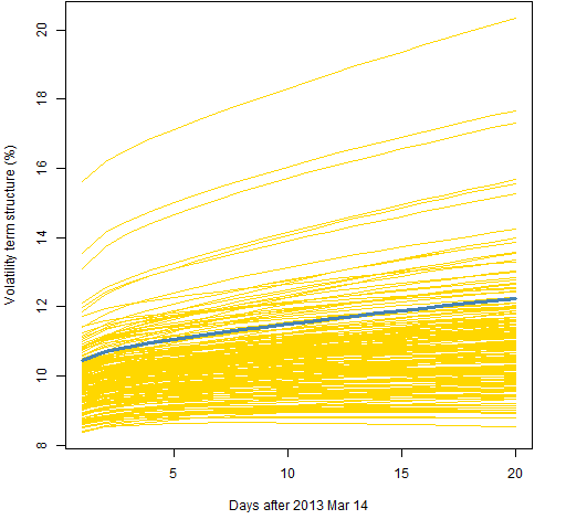
Figure 8: Volatility term structure variability for the component model with t distribution and 500 returns. 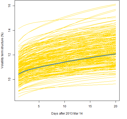 Figure 9 shows the standard deviation of the simulated predictions for the models using 2000 returns.
Figure 9: Standard deviation of simulated predictions with 2000 returns of component-t (blue), component-normal (green), garch(1,1)-t (gold) and garch(1,1)-normal (black). 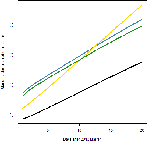 The normal distribution shows less variability than the t distribution. But the t distribution is probably giving us more accurate predictions. The root mean squared difference between the simulated predictions and the original prediction gives a pattern very similar to that of the standard deviation.
Figure 10 shows the standard deviation for the component model with the t distribution for the four different lengths of data.
Figure 10: Standard deviation of simulated predictions of component-t model with 500 returns (gold), 1000 returns (green), 2000 returns (blue) and 5000 returns (black). 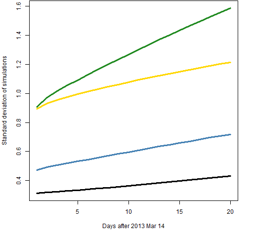 In Figure 10 we expect to see small sample size at the top and big sample size at the bottom. That is violated in that sample size 500 is below 1000. Perhaps this is a sign that our estimate of the variability of variability is very variable.
Questions
What are the weaknesses of this approach to variability?
What are other ways of answering the same question?
What is happening in Figure 10?
Summary
From Figure 10 we have a hint that using much less than 2000 returns can give quite variable results. But increasing the sample size beyond 2000 doesn’t decrease the variability very fast — and the bias of the predictions goes up with the longer samples.
While this technique provides some illumination, it doesn’t give us the full picture.
Appendix R
The computations were done in R. In particular the rugarch package was used.
specifying garch models
I find it hard to remember the form of the garch specification. Here is a little function that makes it easy to create specifications for the four models of interest here:
pp.garchspec <- function(component=TRUE, tdist=TRUE,
    fixed.pars=list())
{
  # convenience to give spec for one of four garch models

  # placed in the public domain 2013 by Burns Statistics

  # testing status: seems to work

  ugarchspec(mean.model=list(armaOrder=c(0,0)),
      distribution=if(tdist) "std" else "norm",
      variance.model=list(model=
      if(component) "csGARCH" else "sGARCH"),
      fixed.pars=fixed.pars)
}
predicted term structure
A function to get predicted volatility term structure is:
pp.garchVolTerm <- function(gfit, ahead=20, annualize=252)
{
  # compute predicted volatility term structure
  # given a garch fit

  # placed in the public domain 2013 by Burns Statistics

  # testing status: untested

  predvar <- ugarchforecast(gfit,  n.ahead=ahead)@
     forecast$forecasts[[1]][, 'sigma']^2
  predterm <- cumsum(predvar) / 1:ahead
  100 * sqrt(annualize * predterm)
}
term structure variability
The function that created the simulated predictions was:
pp.garchVolTermSim <- function(rets, component=TRUE, tdist=TRUE,
    ahead=20, trials=200, burnIn=100, annualize=252)
{
  # predict volatility term structure plus variability via
  # fits of simulated with the estimated garch model

  # placed in the public domain 2013 by Burns Statistics

  # testing status: untested

  spec <- pp.garchspec(component=component, tdist=tdist)
  gfit <- ugarchfit(spec=spec, data=rets)
  ans <- matrix(NA, ahead, trials+1,
     dimnames=list(NULL,  c("real", paste("sim", 1:trials))))
  ans[,1] <- pp.garchVolTerm(gfit, ahead=ahead, annualize=annualize)
  simseries <- as.data.frame(ugarchsim(gfit,
      n.sim=gfit@model$modeldata$T, n.start=burnIn, m.sim=trials),
      which="series")
  for(i in seq_len(trials)) {
    tfit <- try(ugarchfit(spec=spec, data=simseries[,i]))
    if(inherits(tfit, "try-error")) next
    tco <- coef(tfit)
    tco <- tco[!(names(tco) %in% "mu")]
    tspec <- pp.garchspec(component=component, tdist=tdist,
                          fixed.pars=as.list(tco))
    thisfit <- ugarchfit(spec=tspec, data=rets)
    ans[, i+1] <- pp.garchVolTerm(thisfit, ahead=ahead,
       annualize=annualize)
  }
  fails <- sum(is.na(ans[1,]))
  if(fails) {
    warning("There were ", fails,
       " series that failed in estimation")
  }
  attr(ans, "call") <- match.call()
  ans
}
See below for why the call attribute was a good idea.
Technical note: If all of the parameters are fixed when fitting a garch model with ugarchfit, then the result is no longer the same type of object. I’d rather at least have a choice to get back the usual type. In this setting we are fixing all but the mean return. Whether or not that parameter is fixed will have negligible effect on the results.
plotting variability
Figure 2 was created like:
pp.plotVolTermSim(vts.ct.2000, xlab="Days after 2013 Mar 14")
where:
pp.plotVolTermSim <- function(x, xlab="Days ahead",
    ylab="Volatility term structure (%)", ...)
{
  # plot volatility term structure simulation

  # placed in the public domain 2013 by Burns Statistics

  # testing status: untested

  matplot(x, type="l", lty=1, col="gold", xlab=xlab,
     ylab=ylab, ...)
  lines(x[,1], lwd=3, col="steelblue")
}
checking for bugs
Figure 10 produced a surprising result. It certainly could have been because of a mix-up in the objects — either the name of the object or the call that created it was not as intended. But the simulation objects are self-describing in that they have an attribute that shows the command that created them.
Doing the following command:
for(i in ls(pat="^vts")) {cat(i, "\n"); print(attr(get(i), "call"))}
showed that the objects were all created as intended. Hence the surprise lies elsewhere.
