Task
Compute the valuation of a portfolio at one or more times. These can then be plotted.
Preparation
This presumes that you have or can create a portfolio object. For example, that you have mastered “Passive, no benchmark (minimum variance)”.
- portfolio object
- Portfolio Probe
You need a portfolio object with which to create valuations.
You also need to have the Portfolio Probe package loaded into your R session:
require(PortfolioProbe)
If you don’t have Portfolio Probe, see “Demo or Buy”.
Doing the example
opMinVarobject from the “Passive, no benchmark (minimum variance)” examplepprobeDatapackage
You need to have the package loaded into your R session:
require(pprobeData)
Doing it
We do these tasks:
- the valuation at one point in time
- the valuation path through time
Valuation at one point in time
We create the valuation by using prices at the time point of interest:
valOpMinVarEnd07 <- valuation(opMinVar,
   xassetPrices[502,], collapse=TRUE)
This uses the prices at the close of the last trading day of 2007, so one year after the portfolio was formed.
The valuation is:
> format(valOpMinVarEnd07, nsmall=2, big.mark=",")
        prices
"3,090,027.16"
Valuation path through time
Instead of focusing on one specific time, we look at the evolution of value over time.
To do this we need to use a matrix of prices for the times (and assets) of interest:
valOpMinVarDaily07 <- valuation(opMinVar,
   xassetPrices[251:502,], collapse=TRUE)
The result is a vector with a value for each time in the price matrix that we gave to valuation.
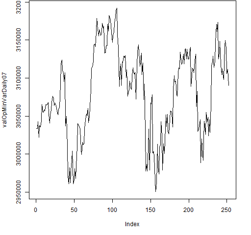
We can just plot the path without trauma:
plot(valOpMinVarDaily07, type="l")
The result of that command is Figure 1.
Figure 1: Default plotting of valuation path. 
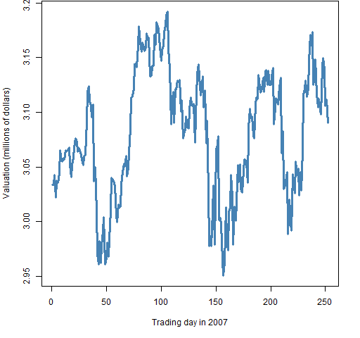
A more pleasing plot can be produced using something like:
plot(valOpMinVarDaily07/1e6, xlab="Trading day in 2007",
   ylab="Valuation (millions of dollars)", , type="l",
   col="steelblue", lwd=3)
The command above produces Figure 2.
Figure 2: More pleasing plot of the valuation path. 
Explanation
The valuation function can do quite a lot. We’ve seen that it can take prices at either one time or multiple times and return something sensible.
The collapse argument controls the granularity of the result. When it is FALSE, then you get information on the individual assets. When it is TRUE, you get information on the portfolio as a whole. (It is possible to have something in between as well.)
Further details
We have given the valuation function an object that was the result of a call to trade.optimizer. But we didn’t need to. We would get the same thing if we gave it a vector that described the portfolio — that is, a vector of the number of units of each asset where the names are the asset identifiers.
In particular, these commands give us the same answer:
valOpt <- valuation(opMinVar, xassetPrices[500:503,],
   collapse=TRUE)
valVec <- valuation(opMinVar$new.portfolio,
   xassetPrices[500:503,], collapse=TRUE)
We compare the two return vectors by binding them into a matrix, and show the vector that we give to valuation in the second instance:
> rbind(valOpt, valVec)
       2007-12-27 2007-12-28 2007-12-31
valOpt    3105810    3111558    3090027
valVec    3105810    3111558    3090027
       2008-01-02
valOpt    3059643
valVec    3059643
> opMinVar$new.portfolio
XA105 XA280 XA298 XA643 XA675 XA709 XA731 XA778
 2659 17920  2906 20192  7182  6485  4166  6840
XA891 XA966
 5200  6247
See also
Navigate
- Back to “Optimize Trades”
- Back to the top level of “Portfolio Probe Cookbook”
