Torturing portfolios to give different volatilities between a factor model and Ledoit-Wolf shrinkage.

Previously

There have been posts on:

• “What the hell is a variance matrix?”
• factor models
• Ledoit-Wolf shrinkage

Question

Two of the several ways to produce an estimate of the variance matrix of asset returns is a statistical factor model and Ledoit-Wolf shrinkage.  Can we learn anything about what is happening when the two estimates give different answers for a portfolio?

We can manufacture such portfolios by generating random portfolios that satisfy some constraints including that the portfolio variances have some minimum difference.

Data

Daily returns during 2012 were used for 442 large cap US stocks.  The variance estimates were based on these returns.

The portfolios were generated as of the end of 2012.  All of the portfolios that were created had the constraints:

• long-only
• exactly 10 assets in the portfolio
• the minimum weight of assets in the portfolio is 0.5%

Many of the portfolios had additional constraints on variance.

All sets of random portfolios consist of 1000 portfolios.

Results

Figure 1 shows the distribution of the volatility for portfolios that obey only the constraints given above.

Figure 1: Distribution of volatility of random portfolios with 10 assets, are long-only and meet the minimum weight constraint. 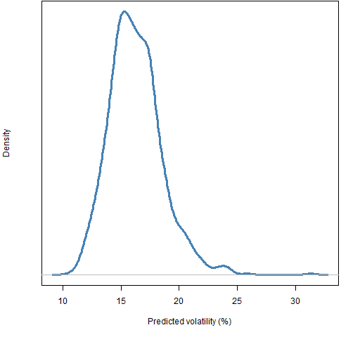The volatility range of 14% to 15% was selected as an additional constraint.  Figure 2 shows the distribution of the difference in estimated portfolio variances for portfolios generated with the basic constraints plus the volatility range.

Figure 2: Distribution of variance differences for portfolios with Ledoit-Wolf volatility between 14% and 15%.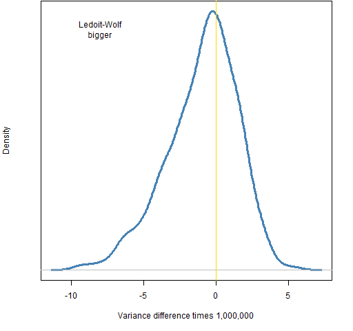 

We see that in this case the factor model is likely to give a smaller estimate of volatility than Ledoit-Wolf. Which one is more likely to have a larger value depends on the particular constraints.  The picture when the factor model is used to estimate volatility is very similar to Figure 2 — that is not always the case with other constraints.

The 10 and -10 on the x-axis is a difference of about 0.8% to 0.9% in volatility for the volatility range we are in.  That is the minimum difference that is imposed for the portfolios that have divergent volatility estimates.

Figure 3 shows the fraction of random portfolios with 14% to 15% Ledoit-Wolf volatility that each asset appears in versus the asset volatility.

Figure 3: Fraction of portfolios in which each asset appears versus the asset volatility for portfolios with 14% to 15% Ledoit-Wolf volatility.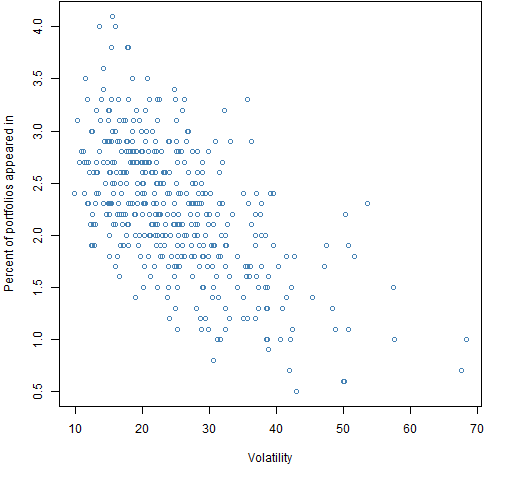

We see that the higher volatility assets are less likely to appear.  This is because the restriction to a volatility of 14% to 15% is below average.  The selection effect is quite mild though.

Figures 4 and 5 compare the volatility estimates for the portfolios that have a difference of variances imposed.

Figure 4: Ledoit-Wolf volatility versus factor model volatility for portfolios with larger Ledoit-Wolf volatility.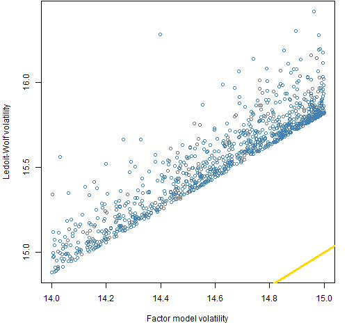

Figure 5: Ledoit-Wolf volatility versus factor model volatility for portfolios with larger factor model volatility. 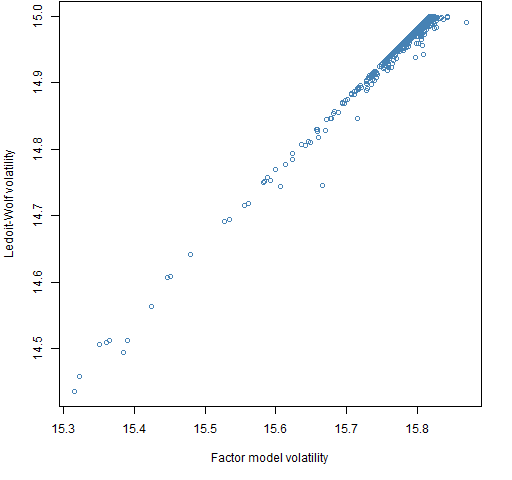In Figure 4 the full range of 14% to 15% volatility is represented with some of the portfolios having a substantially larger difference than the limit imposed.  There is a tendency for portfolios to have a larger volatility (but that is true without the difference constraint).

Figure 5 hints at the difficulty of imposing the difference in this direction.  Only the upper range of volatility is represented, almost all the portfolios are near 15% Ledoit-Wolf volatility, and the difference is never much larger than the minimum imposed.

Figures 6 and 7 show the occurrence of individual stocks in the portfolios with the variance differences imposed.

Figure 6: Fraction of portfolios in which each asset appears versus the asset volatility for portfolios with larger Ledoit-Wolf volatility.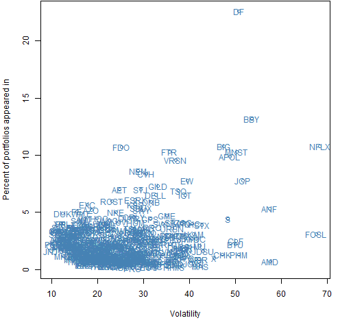

Figure 7: Fraction of portfolios in which each asset appears versus the asset volatility for portfolios with larger factor model volatility. 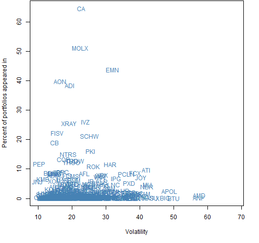There is quite strong selection for particular assets — especially for the larger factor model case.

Below we look at the five most popular assets as shown in Figures 6 and 7 in terms of the diferences in the variance matrix estimates.

Big Ledoit-Wolf popular assets

Ledoit-Wolf variance (for percent returns):

        DF   BBY  NFLX  BIG  FDO
DF   10.20  1.73  0.21 0.85 0.52
BBY   1.73 11.37  2.58 1.47 0.57
NFLX  0.21  2.58 18.52 3.31 1.28
BIG   0.85  1.47  3.31 8.92 1.21
FDO   0.52  0.57  1.28 1.21 2.51

Factor model minus Ledoit-Wolf variance (for percent returns):

        DF   BBY  NFLX   BIG   FDO
DF   -0.04 -1.15  0.25 -0.74 -0.24
BBY  -1.15 -0.04 -1.09 -0.75 -0.21
NFLX  0.25 -1.09 -0.07 -2.12 -0.75
BIG  -0.74 -0.75 -2.12 -0.04 -0.80
FDO  -0.24 -0.21 -0.75 -0.80 -0.01

Ledoit-Wolf correlation:

       DF  BBY NFLX  BIG  FDO
DF   1.00 0.16 0.01 0.09 0.10
BBY  0.16 1.00 0.18 0.15 0.11
NFLX 0.01 0.18 1.00 0.26 0.19
BIG  0.09 0.15 0.26 1.00 0.26
FDO  0.10 0.11 0.19 0.26 1.00

Factor model minus Ledoit-Wolf correlation:

        DF   BBY  NFLX   BIG   FDO
DF    0.00 -0.11  0.02 -0.08 -0.05
BBY  -0.11  0.00 -0.07 -0.07 -0.04
NFLX  0.02 -0.07  0.00 -0.16 -0.11
BIG  -0.08 -0.07 -0.16  0.00 -0.17
FDO  -0.05 -0.04 -0.11 -0.17  0.00

Big factor model popular assets

Ledoit-Wolf variance (for percent returns):

       CA MOLX  EMN  AON  ADI
CA   2.05 0.82 0.54 0.30 0.72
MOLX 0.82 1.99 1.51 0.76 1.10
EMN  0.54 1.51 4.05 1.07 1.30
AON  0.30 0.76 1.07 1.08 0.66
ADI  0.72 1.10 1.30 0.66 1.50

Factor model minus Ledoit-Wolf variance (for percent returns):

        CA MOLX   EMN   AON  ADI
CA   -0.01 0.11  0.47  0.20 0.10
MOLX  0.11 0.11  0.21  0.07 0.15
EMN   0.47 0.21 -0.02 -0.03 0.13
AON   0.20 0.07 -0.03  0.00 0.02
ADI   0.10 0.15  0.13  0.02 0.09

Ledoit-Wolf correlation:

       CA MOLX  EMN  AON  ADI
CA   1.00 0.41 0.19 0.20 0.41
MOLX 0.41 1.00 0.53 0.52 0.64
EMN  0.19 0.53 1.00 0.51 0.53
AON  0.20 0.52 0.51 1.00 0.52
ADI  0.41 0.64 0.53 0.52 1.00

Factor model minus Ledoit-Wolf correlation:

       CA MOLX   EMN   AON  ADI
CA   0.00 0.04  0.16  0.14 0.05
MOLX 0.04 0.00  0.06  0.03 0.05
EMN  0.16 0.06  0.00 -0.01 0.04
AON  0.14 0.03 -0.01  0.00 0.00
ADI  0.05 0.05  0.04  0.00 0.00

Questions

Anyone see any significance in the assets that are selected for in the portfolios with big differences?

Summary

The differences in correlation estimates seem to be driving the differences in portfolio volatility estimates.  Given that there are almost 100,000 correlations, the correlation differences that have the largest impact don’t seem all that big.

Portfolios with 10 assets are more likely to have large discrepancies than larger portfolios.  Hence it seems unlikely that volatility estimates for real portfolios will differ much between the two methods.

Epilogue

Both of us say there are laws to obey
But frankly I don’t like your tone

from “Different Sides” by Leonard Cohen

Appendix R

Computations and plots were done in R.

variance estimation

The two variance estimates use functions from the BurStFin package.

require(BurStFin)

fm12 <- factor.model.stat(initret12)
lw12b <- var.shrink.eqcor(initret12, tol=1e-5)

As “Correlations and positive-definiteness” points out, the default value of the tol argument in the Ledoit-Wolf estimate is over zealous about making sure that there are no portfolios estimated to have very small variance.  (The default will be changed when the package is updated.)

generate wild portfolios

The generation and manipulation of the random portfolios depends on the Portfolio Probe package.  1000 portfolios with just the initial three constraints are generated with:

require(PortfolioProbe)

rp10wild <- random.portfolio(1000, priceEnd12, 
   port.size=c(10,10), gross=1e6, long.only=TRUE, 
   min.weight.thresh=.005)

There is an additional constraint in the command that the gross value needs to be close to $1 million.  While a specification of the amount of money in the portfolios is mandatory, it has no effect on our results (unless the amount is tiny).

The min.weight.thresh argument is new in Portfolio Probe version 1.06.

get volatility

The volatility estimate for each of the portfolios is produced with:

vol.rp10wild <- sqrt(unlist(randport.eval(rp10wild, 
   keep="var.values",
   additional.args=list(variance=lw12b))) * 252) * 100

This first produces a vector of the Ledoit-Wolf estimates of the variance of each portfolio, and then transforms that into volatility.

generate volatility restricted portfolios

We want to restrict volatility to the range of 14% to 15%.  However, the software thinks in terms of variance rather than volatility.  So we need to transform to the variance scale that we have.  We also need the bounds for the variance constraint to be a two-column matrix:

vcmat1 <- matrix(c(.14, .15)^2/252, 1, 2)

Now we use this matrix:

rp10vtest <- random.portfolio(1000, priceEnd12, 
   port.size=c(10,10), gross=1e6, long.only=TRUE, 
   min.weight.thresh=.005, variance=lw12b, 
   var.constraint=vcmat1)

see variance differences

Now we can see what the difference is between the two variance estimates for each of these portfolios:

vardif.rp10vtest <- unlist(randport.eval(rp10vtest, 
   keep="var.values",
   additional.args=list(variance=fm12-lw12b, 
      var.constraint=NULL)))

We change what it thnks the problem is by putting in a different value for the variance matrix and removing the variance constraint.

You may be wondering if the difference of variance matrices really gives us the portfolio variance differences.  The portfolio variance is the double sum over assets of the (i,j) position in the variance matrix times the i-th weight times the j-th weight.  So it is linear in the variance matrix values.

count assets in portfolios

The command to count how many times each asset appears in a portfolio is:

acount.rp10vtest <- table(sapply(rp10vtest, names))

generate variance difference portfolios

Now we know what variance differences are feasible.  We want to impose two different variance constraints:

• volatility is 14% to 15% (according to one of the variance matrices)
• the difference of variances is at least 1e-5

To do this we need to provide two variance matrices in the form of a three-dimensional array, where each slice of the third dimension is a variance matrix.  We also need a constraint on each of the variances.  So we need a 2 by 2 matrix: columns are minimum and maximum allowed, rows are for the different variances.

vcmat2 <- rbind(vcmat1, c(1e5, Inf))

The random portfolios are generated with:

rp10biglw <- random.portfolio(1000, priceEnd12, 
   port.size=c(10,10), gross=1e6, long.only=TRUE, 
   min.weight.thresh=.005, 
   variance=threeDarr(fm12, lw12b-fm12), 
   var.constraint=vcmat2)

The threeDarr function is in the BurStFin package and it stacks matrices into a three-dimensional array.

difficult constraints

Figure 2 shows that the variance difference where Ledoit-Wolf is bigger (what the command above is getting) is rare, but not exceedingly rare.  But we might think that the difference where the factor model is bigger could be impossible.  As Figure 5 shows, it isn’t impossible but barely.

When generating random portfolios, you want it to give up trying if it can’t find any within a reasonable amount of time — you don’t want to have to throw your computer away every time you ask it to do something impossible.  The default settings suggested that the factor-model-bigger problem was impossible.  Changing the settings so it worked harder on each try, and was less frustrated with failure allowed the generation to go ahead.

The time to generate random portfolios heavily depends on the constraints.  To get 1000 portfolios that satisfied the Ledoit-Wolf bigger constraint took 5 seconds.  To get the factor model bigger constraint it took just under 23 hours.

selected variances and correlations

To get the most selected names:

acnam.biglw <- rev(names(tail(sort(acount.rp10biglw),5)))

Variance matrix selection was:

round(lw12b[acnam.biglw, acnam.biglw] * 1e4, 2)

Correlation matrix selection was:

round(cov2cor(lw12b[acnam.biglw, acnam.biglw]), 2)