What to expect from fund managers who follow your investment mandate.

You hope that the fund managers that you hire have skill.  But markets are noisy so it is hard to tell skill from luck.  It is impossible to tell skill from luck if you don’t know what luck looks like.

Here we draw pictures of what luck looks like for past periods of time.  The technique is to create a large number of portfolios that obey the rules of the mandate but are otherwise random, and then draw the distribution of their returns.

Crude example

Suppose the mandate is:

• The universe is the equities in the S&P 500
• The portfolio is long-only
• There are to be at least 60 and no more than 100 names in the portfolio
• No weight at rebalancing time is to be greater than 2.5%

Figures 1 through 4 show the distribution of luck for each of the quarters in 2012.  Figure 5 shows the luck distribution when the portfolios formed at the start of 2012 are held for the full year.  Finally Figure 6 shows the distribution for the first quarter of 2013.  Simple returns are reported in all cases.

Figure 1: Distribution of returns in 2012 Q1 of random portfolios following the mandate.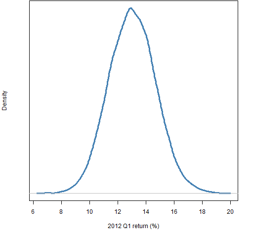

Figure 2: Distribution of returns in 2012 Q2 of random portfolios following the mandate.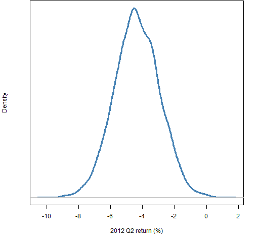

Figure 3: Distribution of returns in 2012 Q3 of random portfolios following the mandate.

Figure 4: Distribution of returns in 2012 Q4 of random portfolios following the mandate.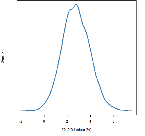

Figure 5: Distribution of returns in 2012 of random portfolios following the mandate.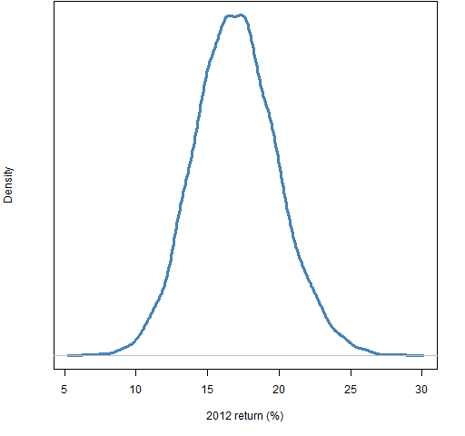

Figure 6: Distribution of returns in 2013 Q1 of random portfolios following the mandate.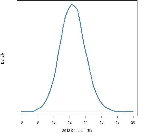

The information can be used in ways beyond just drawing pictures.  For example, if a manager you hired with this mandate had a 15% return during the first quarter of 2013, you could find that only about 5% of the random portfolios did better than that.

Note that “expectation” is statistical jargon for the mean.  We are using “expected” in the non-technical sense of “typical” (with zero skill).

What you need

You don’t need very much to do this sort of exercise yourself.

In addition to software that will generate random portfolios, you need prices of the assets in the universe at the ends of the periods that you are interested in.

You also need information that is required to form the constraints in the mandate.  If you have sector constraints, then you need the sector classifications.  If you have a tracking error constraint, then you need the weights for the benchmark and a variance matrix for the returns of the assets in the universe.

Even better

There are more nuanced ways of looking at the performance of a particular fund.  These are more labor-intensive but can provide much more insight into the fund.  The fund manager is in the best position to do those analyses.

There is an easy approximation to these analyses though:  Generate random portfolios that obey the mandate constraints where the starting portfolio is specified to be the portfolio held by the fund at the start of the period and the turnover is constrained to be close to the realized or expected amount of turnover for the fund.

Appendix R

The figures and the computing for them were done with R.

preparation

The only data that was required for the example was a matrix of prices for the universe (actually 443 stocks were used, some of which may have fallen out of the index by now).  Times are in the rows and each column is a different stock.

This is a matrix of daily closing prices, but we are only interested in a few of those days — 6 days to be exact.  To discover which are the rows we care about, a trick was used to see where 2012 and 2013 start.  It went like:

yearSwitch <- which(diff(as.numeric(substring(
  rownames(univclose130406), 1, 4))) > 0)

This extracts the year (first four characters) from the row names, coerces that from character to numeric, finds the difference of each element from the previous element, and sees where those differences aren’t zero.

The same sort of thing could have been done with months to find the places of the dates of interest, but since there were only a few, it was just as easy to do some experimenting by hand.  The result was a vector of the row numbers of the dates of the last day of 6 quarters:

qtimes1213 <- c(2015, 2077, 2140, 2203, 2265, 2325)

Below we use this vector to subscript the original matrix of prices.  Another option would have been to create a new matrix with just those 6 rows.

generate portfolios

Five sets of random portfolios were generated using the closing prices on the day before the start of each quarter in 2012 and the first quarter in 2013.  The command to do the first was:

require(PortfolioProbe)

rp12q1 <- random.portfolio(number.rand=1e4, 
   prices=univclose130406[qtimes1213[1], ], 
   long.only=TRUE,gross=1e6, port.size=c(60,100), 
   max.weight=.025)

This specifies the constraints in the mandate.  It also sets the amount of money in each portfolio to very close to one million dollars — that is immaterial to the returns.  10,000 portfolios were generated for each set.

compute returns

The returns of the random portfolios were found with commands like:

retrp12q1 <- valuation(rp12q1, 
   prices=univclose130406[qtimes1213[1:2],],
   returns="simple")
retrp12all <- valuation(rp12q1, 
   prices=univclose130406[qtimes1213[c(1,5)],],
   returns="simple")
retrp12q2 <- valuation(rp12q2, 
   prices=univclose130406[qtimes1213[2:3],],
   returns="simple")

plot distributions

The simple command to plot the distribution of returns is:

plot(density(retrp12q1))

The actual command that created Figure 1 was:

plot(density(retrp12q1 * 100), lwd=3, col="steelblue", 
   yaxt="n", main="", xlab="2012 Q1 return (%)")

compute percentile

The computation with the example of a 15% return in 2013 Q1 was:

> mean(retrp13q1 < .15) 
[1] 0.9494