Here we give details and code for the prediction distributions exhibited in yesterday’s blog post “Tis the season to predict”.
[Revision: There was a problem with the plots published in that post. For corrected plots and an explanation of the error, see Revised market prediction distributions.]
Eight years of returns
The equity indices use daily closing levels from the start of 2003. This data comes from Yahoo.
A roughly equivalent technique of selecting the last 2000 daily prices is used for oil. The data are from the U. S. Energy Information Administration.
Then log returns are created.
Estimating market trend
Since the idea of what we are doing is to predict assuming the underlying market doesn’t move, we need to find an estimate of the market moves. The method chosen was to use the loess R function with a span of 7 observations.
This yields an extremely volatile trend.
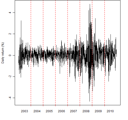
Figure 1: The estimated trend for FTSE 100 (daily scale).
To emphasize just how extreme this is, Figure 2 is the same as Figure 1 except the scale is annual returns.
Figure 2: The estimated trend for FTSE 100 (annual scale).
This is pretty much as volatile as we would want to go with loess. When the span is reduced to 5 observations, about half of the residuals are zero. I’m sure there is a perfectly good explanation for this, but I don’t know what it is.
The extreme roughness of the trend means that we are erring on the side of too small of moves in the simulations.
GARCH model
An important feature of market data is volatility clustering — there are periods of low volatility and periods of high volatility. We can use garch to model volatility clustering and then simulate that model into the future.
Usually we would feed the returns to the garch model. In this case we instead feed it the residuals from the loess model. These are less volatile than the returns.
We use a GARCH(1,1) model fit with the garch function from the tseries R package. This assumes a normal distribution.
Simulation
The key feature of the simulation that we want is to start the simulation with the current state. In the case of GARCH(1,1) this means the simulation’s starting volatility is the final volatility in the model that was fit.
We use the empirical standardized residuals from the garch model in the simulation (as opposed to assuming a particular distribution).
Since we are keen to remove as much motion as possible, the standardized residuals are symmetrized. That is, each standardized residual is used with an arbitrary sign. Hence zero is both the mean and the median of the distribution.
5000 simulations are performed that each yield a return over the year (actually 250 trading days). The five smallest returns and the five largest returns are removed.
Then the remaining returns are transformed to a level and the density is plotted. In order to keep all of the pictures reasonably proportioned, the top limit of the density is restricted to be no more than three times the initial value.
Criticism
No modeling is perfect. Here we discuss weaknesses and strengths of what was done.
Detrending
The detrending has surprisingly little effect on the width of the prediction distributions. Just extracting a single mean produces distributions that are only moderately wider than those displayed in yesterday’s post. Using a span of 5 rather than 7 creates a lot of zeros in the residuals yet hardly changes the prediction distributions at all.
This insensitivity should give us more faith that the distributions we are seeing are about right. The idea of them being right might make us a little queasy about the operation of markets.
GARCH(1,1)
The GARCH(1,1) model was used because it is the most convenient. It is certainly not the best model.
I don’t know what effect using a better model would have. (One example of a better model would be a components model with a leverage effect and assuming a t distribution.) My guess is that it would have very little effect, but I’ve been wrong before.
Explosive estimates
If the sum of the two garch parameters is greater than 1, then the asymptotic variance of the process is infinite. Some of the estimated models did have this property.
However, there is not much difference between the prediction distributions produced by explosive versus non-explosive models. That — amazingly — doesn’t seem to be a big issue.
Long upper tail
Even the non-explosive models produce prediction distributions with very long upper tails. So some of the paths are explosive even though the model is not. This is even with the most extreme 0.1% paths ignored.
There really could be a long upper tail due to inflation taking off. However, these models know nothing about inflation so that is not what is happening here.
Summary
The tails of the prediction distributions are definitely suspect — 1% and beyond. The central parts are probably reasonably truthful.
Appendix R
You can get the R functions that are used to create the prediction distributions with the R command:
> source('https://www.portfolioprobe.com/R/blog/prediction_dist_funs.R')
Likewise you can get the function that was used to create Figures 1 and 2 in this post with the command:
> source('https://www.portfolioprobe.com/R/blog/pp.timeplot.R')
The commands to create the prediction distribution plots are in prediction_dist.Rscript.

Pingback: Momento R do dia « De Gustibus Non Est Disputandum
Pingback: Algorithmic Trading in R: Available Information « xmphforex
Dear Pat, thanks for sharing your approach. I have a question.
How do you evaluate this predictions?
I have seen some alternatives such as the PITS probability integral transforms, and also the use of the Kullback-Leibler IC. Could you give us some hint how to implement these in R? I would really appreciate your help.
Thanks,
I’d have to start from zero for those. So the first thing I would do would be to search R for them — probably using Rseek. If I wasn’t satisfied, then I’d write a question to Stackoverflow or r-help (that would include a summary of what I had done so far). Good luck.