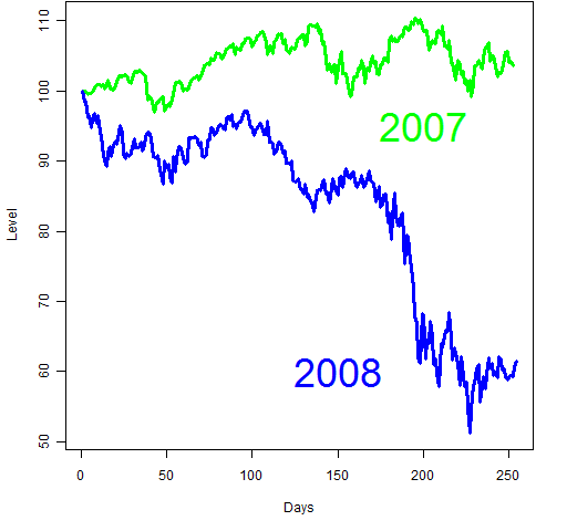
We know that the S&P 500 was up a little in 2007 and down a lot in 2008. So on the surface the question seems really stupid. But randomness played a part. Let’s have a go at deciding how much of a part.
Figure 1: Comparison of 2007 and 2008 for the S&P 500.
Statistical bootstrap
The bootstrap is an easy way to find the variability of a statistical procedure. (Easy, that is, if you have an appropriate computing environment, such as R.) The idea is to recompute your procedure over and over again using samples from your original data.
We get the annual log return by summing the daily log returns (see A tale of two returns). So we can do a bootstrap for this in R like:
> bs07 <- numeric(10000)
> for(i in 1:10000) bs07[i] <- sum(sample(spx07,
+ 251, replace=TRUE))
> plot(density(bs07)) # essentially Figure 2
Figure 2: Bootstrap distribution for S&P 500 for 2007.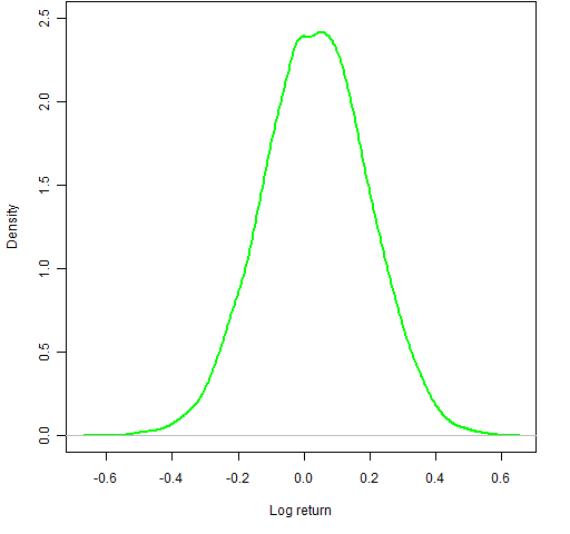
You can use the multiverse interpretation to understand Figure 2. We are looking at ten thousand different universes — each of them has the same distribution of daily returns as our universe in 2007. Some universes are lucky, some are not.
Figure 3: Bootstrap distributions for the S&P 500 for each of 2007 and 2008.
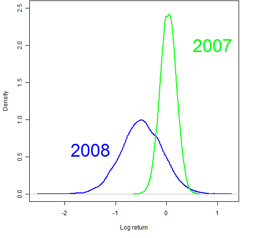
Figure 3 shows the bootstrap distributions of both 2007 and 2008. The spread for 2008 is amazing. Some of the most extremely low values lost about 80% of the value (a simple return of –.8 corresponds to a log return of about –1.6). I’m intrigued with the other extreme: 2008 has more mass on the right than 2007.
Volatility was much higher in 2008 than 2007. That is why the 2008 distribution is so much wider.
Figure 4: Bootstrap distribution of year 2007 minus year 2008.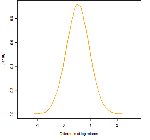
Figure 4 shows the return in 2007 minus the return in 2008 for each of the ten thousand universes. Our presumption is that this should be unambiguously above zero. It isn’t — about 12% of the distribution is below zero.
Assumptions
One of the really nice things about the bootstrap is that there is a minimum of assumptions. The one key assumption that it does have is that the data are independent and identically distributed.
Our return data are not independent and identically distributed.
We know for sure that there is volatility clustering — periods of low volatility and periods of high volatility. A lot of people presume that the expected value of the return changes over time as well — that there are bull and bear markets. Belief in that may make it true even if it weren’t already true.
Model expected returns
One approach of handling the problem of changes in expected returns is to use the loess nonparametric regression in R — we estimate expected return for each point in time. This doesn’t take care of volatility clustering, but that is much less problematic for the inference that we are trying to make.
Figure 5: Two loess views of expected returns.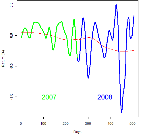
The red line in Figure 5 shows the default loess fit. The other line uses robust estimation and much less smoothing. This is probably about as wiggly of a line as we would want. We see that at the worst point, it is expecting the return to be less than -1% per day.
We can use the fit and residuals from this model to do bootstrapping again. The resulting bootstrap distributions are virtually identical to the original ones. Figure 6 gives a hint of why this is the case.
Figure 6: 2008 loess residuals compared to the returns.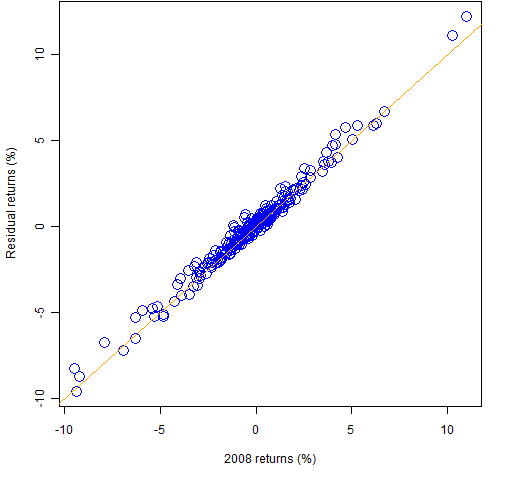
Figure 6 shows that the distribution of the residuals (from the wiggly fit) and the original returns are not very different. The extreme negative fit is associated with large positive returns as well as large negative returns. We haven’t managed to squeeze much noise into signal.
Conclusion
Surprisingly, we haven’t found much evidence that 2007 was really better than 2008. Perhaps someone else sees a clever way of partitioning signal and noise.
Epilogue
Here is more on statistical bootstrapping and its relatives.
Appendix R
> spxdf <- data.frame(days=1:504, ret=c(spx07, spx08))
> losym10 <- loess(ret ~ days, data=spxdf,
+ family="symmetric", span=.1)
The first line above creates a suitable data frame consisting of a column that is the number of trading days from the start of 2007 and a column that is the daily returns.
The second line fits the loess model using a span of 10% of the data (instead of the default of 75%) and using the symmetric family rather than the gaussian family. This is the fit that appears prominently in Figure 5.
The return data are now available as two R objects: spx07 and spx08
You can put these into your global environment in R with:
load(url(
'https://www.portfolioprobe.com/R/SandP_0708.rda'))
Pingback: Blog year 2010 in review | Portfolio Probe | Generate random portfolios. Fund management software by Burns Statistics